THESIS
Kernel Methods and Frequency Domain Independent Component Analysis for
Robust Speaker Identification
Submitted by Makoto Yamada
Department of Statistical Science
In partial fulfillment of the requirements For the Degree of Doctor of Philosophy The Graduate University for Advanced Studies
Hayama, Japan Mar 2010
THE GRADUATE UNIVERSITY FOR ADVANCED STUDIES
Mar, 2010 WE HEREBY RECOMMEND THAT THE THESIS PROPOSAL PREPARED UNDER OUR SUPERVISION BY MAKOTO YAMADA ENTITLED KERNEL METHODS AND FREQUENCY DOMAIN INDEPENDENT COMPO- NENT ANALYSIS FOR ROBUST SPEAKER IDENTIFICATION BE AC- CEPTED AS FULFILLING IN PART REQUIREMENTS FOR THE DEGREE OF DOCTOR OF PHILOSOPHY.
Committee on Graduate Work
Prof. Kenji Fukumizu
Prof. Shiro Ikeda
Prof. Masashi Sugiyama
Prof. Tomoko Matsui Adviser
Prof. Takashi Tsuchiya
Department Head/Director
ABSTRACT OF THESIS
Kernel Methods and Frequency Domain Independent Component Analysis for Robust Speaker Identification
The speaker identification is one of the key technologies for person identification in humanoid robots. Especially, when the face information is not available, the speaker identification is the only way to identify person, thus, to improve the speaker identi- fication performance is an important issue for person identification tasks.
There are four major issues in speaker identification for humanoid robots in prac- tice. First, the humanoid robots should identify the speaker in real-time with high identification rates. In these days, the kernel methods such as the support vector machine (SVM) and kernel logistic regression (KLR) are popular for speaker identifi- cation tasks, and the kernel based systems outperform the conventional Gaussian Mixture Model (GMM) based system. However, the kernel based speaker iden- tification systems are usually computationally intensive, and this is of course not preferable for real-time implementation. To deal with the computational issue, we propose a method of approximating the sequence kernel that is shown to be compu- tationally very efficient in Chapter 3. More specifically, we formulate the problem of approximating the sequence kernel as the problem of obtaining a pre-image in a reproducing kernel Hilbert space. The effectiveness of the proposed approximation is demonstrated in text-independent speaker identification experiments with 10 male speakers—our approach provides significant reduction in computation time while per- formance degradation is kept moderately. Based on the proposed method, we develop
a real-time kernel-based speaker identification system using the Virtual Studio Tech- nology (VST).
Second, the speech features vary over time due to session dependent variation, the recording environment change, and physical conditions/emotions. However, con- ventional kernel based systems implicitly ignore these facts, and they just simply assume that the training and test input probability distributions of the training and test datasets are same at any time. To alleviate the influence of session dependent variation, it is popular to use several sessions of speaker utterance samples or to use cepstral mean normalization (CMN). However, gathering several sessions of speaker utterance data and assigning the speaker ID to the collected data are expensive both in time and cost and therefore not realistic in practice. Moreover, it is not possi- ble to perfectly remove the session dependent variation by CMN alone. Thus, in Chapter 4, we propose a novel semi-supervised speaker identification method that can alleviate the influence of non-stationarity such as session dependent variation, the recording environment change, and physical conditions/emotions. We assume that the voice quality variants follow the covariate shift model, where only the voice feature distribution changes in the training and test phases. Our method consists of weighted versions of kernel logistic regression and cross validation and is theoretically shown to have the capability of alleviating the influence of covariate shift, where the weight (a.k.a importance) is estimated from the training and test distribution using the Kullback-Leibler Importance Estimation Procedure (KLIEP). We experimentally show through text-independent/dependent speaker identification simulations that the proposed method is promising in dealing with variations in voice quality.
Third, the humanoid robots are desired to automatically detect the unknown speaker and add the unknown speaker into the dictionary. Thus, the speaker detec- tion task can be formulated as the outlier detection problem (i.e., outliers can be the unknown speakers). Since the outlier detection problem can be solved through the
comparison between the log likelihoods of the unknown speaker and the speakers, the estimation accuracy of the log likelihoods is an important issue to improve the speaker detection performance. Thus, in Chapter 5, we propose a new importance (a.k.a likelihood) estimation method using Gaussian mixture models (GMMs) and principal component analyzers (PPCAs) mixture, where the proposed approach esti- mates the importance without going through the density estimation. An advantage of the proposed methods is that covariance matrices or projection matrices can also be learned through an expectation-maximization procedure, so the proposed method ex- pected to work well when the true importance function has high correlation. Through experiments of outlier detection, we show the validity of the proposed approaches.
Forth, the humanoid robots move throughout the world, and the surrounding environment, source positions, and source mixtures are constantly changing. In ad- dition, the speech overlaps are frequently occurred during conversation. Thus, the source separation techniques are useful for improving the speaker identification per- formance. To deal with those problems, in Chapter 6, we consider the problem of two-source signal separation from a two-microphone array, where a point source such as a speech signal is placed in front of a two-microphone array, while no information is available about another interference signal. We propose a simple and computation- ally efficient method for estimating the geometry and source type (a point or diffuse) of the interference signal, which allows us to adaptively choose a suitable unmixing matrix initialization scheme. Our proposed method, noise adaptive optimization of matrix initialization (NAOMI), is shown to be effective through source separation and speaker identification simulations.
Makoto Yamada Department of Statistical Science The Graduate Universities for Advanced Studies Hayama, Kanagawa, Japan Mar. 2010
ACKNOWLEDGEMENTS
I would like to express my gratitude to my adviser, Dr. Tomoko Matsui, for her helpful support. She has lead me to challenge the real-world problems and made me question things to allow me to obtain a deeper understanding. In addition, I fairly appreciate that she held the research meeting on weekends, because of my inconvenience. Her support has allowed me to be here and has forced me to use all my skills to solve problems.
I also would like to express my gratitude to Dr. Masashi Sugiyama for his supervi- sion in Tokyo Institute of Technology. With his valuable assistance and heartwarming encouragement in spite of his extremely busy schedule, I could enjoy doing research and find many interesting research topics. In addition, I would like to thank Dr. Peter J. Brockwell for encouragement to obtain Ph.D. Without meeting him, I would never challenge to obtain a Ph.D.
I would like to thank my committee members, Dr. Kenji Fukumizu and Dr. Shiro Ikeda, for their patience and cooperation. I also would like to thank my co-authors, Dr. Ali Pezeshki, Dr. Mahmood Azimi-Sadjadi, for valuable discussions, brilliant ideas, and helpful support.
I must deeply thank Hitachi Corporation and Yamaha Corporation for the ap- proval of my study in Matsui laboratory. I would like to express my gratitude to Mr. Furugaki, Mr. Shigeki Fujii, Mr. Hideki Kenmochi, managing director, Mr. Kazunobu Kondo, senior engineer. I am obliged to all the other people working for Yamaha as well. I also would like to thank my friends Juan Jesus Cabrera, Sungyoung
Kim, Gordon Wichern, Fernando V. Marquez, Vincent Wong, Yuu Takahashi, and Yoshikazu Yokotani for encouraging me to obtain Ph.D.
Last but not least, I would like to express my gratitude to my family. I am very grateful to my parents, uncle, and grandparents, for the education they gave me. Special thanks go to my wife, Noriko, for her support, encouragement, and patience during my Ph.D. period.
TABLE OF CONTENTS
SIGNATURE . . . ii
ABSTRACT OF THESIS . . . iii
ACKNOWLEDGEMENTS . . . vi
1 INTRODUCTION . . . 1
1.1 Four issues in Speaker Identification for humanoid robots . . . 1
1.2 Kernel based real-time speaker identification with Acceleration of Mean Operator Sequence Kernel Computation . . . 2
1.3 Semi-supervised Speaker Identification under Covariate Shift . . . . 4
1.4 Direct Importance Estimation using Gaussian Mixture Models and Probabilistic Principal Component Analysis . . . 5
1.5 Noise Adaptive Optimization of Matrix Initialization . . . 7
1.6 Organization of this dissertation . . . 9
2 KERNEL-BASED SPEAKER IDENTIFICATION . . . 10
2.1 Problem formulation . . . 10
2.2 Feature Extraction . . . 11
2.3 Kernel Logistic Regression . . . 12
2.4 Mean Operator Sequence Kernel . . . 15
2.5 Model selection in Kernel Logistic Regression . . . 16
3 KERNEL BASED REAL-TIME SPEAKER IDENTIFICATION WITH ACCELERATING SEQUENCE KERNEL COMPUTATION 18 3.1 Introduction . . . 18
3.2 Problem Formulation . . . 19
3.2.1 Kernel-based Text-independent Speaker Identification . . . . 19
3.2.2 Mean Operator Sequence Kernel [1] . . . 20
3.3 Approximation of MOSK . . . 21
3.3.1 Approximating Mean Operator Sequence Kernel by Parts . . 21
3.4 Experiments . . . 23
3.4.1 System and Data Acquisition . . . 23
3.4.2 Results . . . 24
4 SEMI-SUPERVISED SPEAKER IDENTIFICATION UNDER CO- VARIATE SHIFT . . . 27
4.1 Introduction . . . 27
4.2 Problem Formulation . . . 29
4.2.1 Kernel-based Speaker Identification . . . 29
4.2.2 KLR, CV, and Covariate Shift . . . 31
4.3 Importance Weighting Techniques for Covariate Shift Adaptation . . 32
4.3.1 Parameter Learning and Model Selection under Covariate Shift 32
4.3.2 Importance Weight Estimation . . . 34
4.3.3 Illustrative Examples . . . 35
4.4 Experiments . . . 36
4.4.1 Data and System Description . . . 36
4.4.2 The Results of Speaker Identification under Covariate Shift . 39 5 DIRECT IMPORTANCE ESTIMATION WITH GAUSSIAN MIX- TURE MODEL AND PRINCIPAL COMPONENT ANALYZERS 43 5.1 Introduction . . . 43
5.2 Background . . . 45
5.2.1 Problem Formulation . . . 45
5.2.2 Kullback-Leibler Importance Estimation Procedure . . . 46
5.2.3 Model Selection by Likelihood Cross Validation . . . 47
5.3 KLIEP with Gaussian Mixture Models . . . 48
5.3.1 Derivation of the EM Algorithm . . . 49
5.4 KLIEP with Mixture of Probabilistic Principal Component Analyzers 50 5.5 Experiments . . . 52
5.5.1 Illustrative Example for GM-KLIEP . . . 52
5.5.2 Illustrative Example . . . 54
5.5.3 Application to Inlier-based Outlier Detection . . . 56
6 NOISE ADAPTIVE OPTIMIZATION OF MATRIX INITIALIZA- TION . . . 58
6.1 Introduction . . . 58
6.2 Problem formulation . . . 59
6.2.1 Frequency Domain Independent Component Analysis . . . . 60
6.2.2 Beamformer based unmixing matrix initialization . . . 61
6.3 Noise Adaptive Optimization of Matrix Initialization . . . 63
6.3.1 Estimating the geometry of the interfering sound source . . . 63
6.3.2 Source type classification . . . 65
6.4 Source Separation Experiments . . . 66
6.4.1 point source + point source separation in an anechoic chamber 67 6.4.2 point source + point source separation in reverberant room . 68 6.4.3 point source + diffuse source separation in reverberant room 70 6.4.4 Environmental adaptation in reverberant room . . . 71
6.4.5 Speaker Identification Experiments . . . 73
7 CONCLUSION . . . 75
7.1 Future works . . . 77 7.1.1 Mean Operator Sequence kernel based speaker identification . 77
7.1.2 Semi-supervised speaker identification . . . 77 7.1.3 Direct Importance Estimation . . . 78 7.1.4 Noise Adaptive Unmixing Matrix Initialization . . . 78
LIST OF TABLES
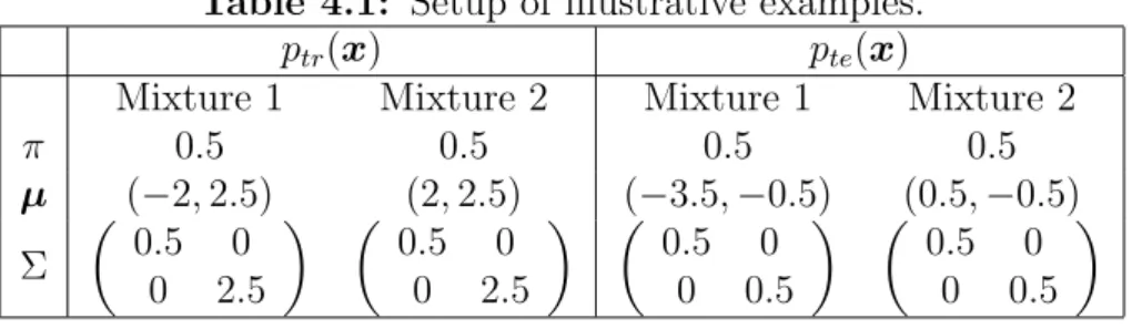
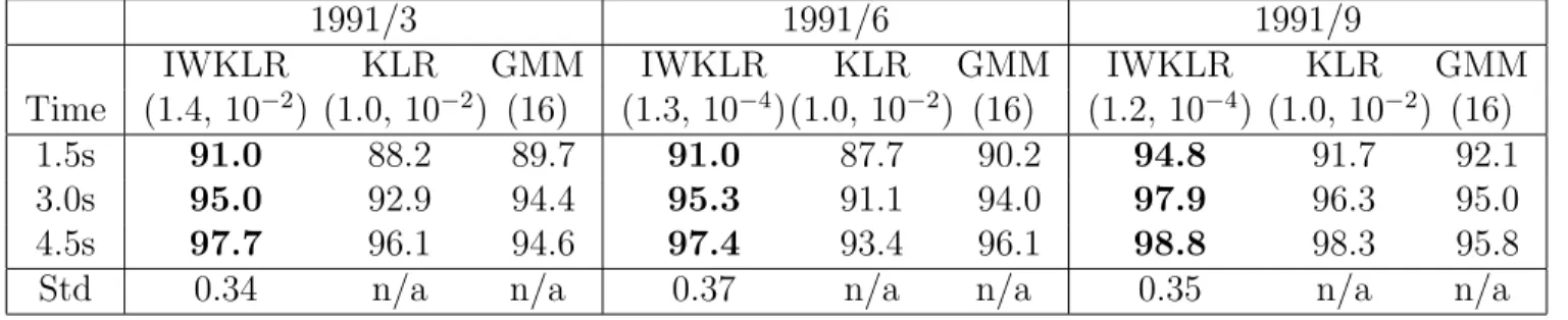
3.1 Training sentences and test words (in Japanese, written using the Hep- burn system of Romanization). . . 24 4.1 Setup of illustrative examples. . . 36 4.2 Correct classification rates for text-independent speaker identification.
All values are in percent. IWKLR refers to IWKLR with σ and δ chosen by 5-fold IWCV, KLR refers to KLR with σ and δ chosen by 5-fold CV, and GMM refers to GMM with the number of mixtures chosen by 5-fold CV. The chosen values of these hyper-parameters are described in the bracket. ‘Std’ refers to the standard deviation of estimated importance weights {w(Xi)}ni=1tr, roughly indicating the degree of distribution change. . . 42 4.3 Correct classification rates for text-dependent speaker identification.
All values are in percent. IWKLR refers to IWKLR with σ and δ chosen by 5-fold IWCV, KLR refers to KLR with σ and δ chosen by 5-fold CV, and GMM refers to GMM with the number of mixtures chosen by 5-fold CV. The chosen values of these hyper-parameters are described in the bracket. ‘Std’ refers to the standard deviation of estimated importance weights {w(Xi)}ni=1tr, roughly indicating the degree of distribution change. . . 42
5.1 Mean AUC values (with their standard deviation in brackets) over 20 trials in the outlier detection experiments. If the performance of one of three methods is significantly different by the t-test at a significance level of 5%, we use ‘◦’ as the case where GM-KLIEP or PM-KLIEP outperforms KLIEP, ‘+’ as the case where KLIEP or PM-KLIEP out- performs GM-KLIEP, and ‘⋆’ as the case where KLIEP or GM-KLIEP outperforms PM-KLIEP. . . 57 6.1 Recording conditions in anechoic chamber . . . 68 6.2 DOA result when the unknown source is directional signal. The mean
and standard deviation of bθ2 are from 30 combinations of speakers. . 68 6.3 DOA result when the unknown source is directional signal. The mean
and standard deviation of bθ2 are from 30 combinations of speakers. . 70 6.4 Speaker identification under environmental change. . . 74
LIST OF FIGURES
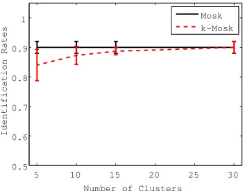
2.1 Feature extraction from a speech signal. . . 12 3.1 Speaker identification rates obtained using 30, 15, 10, and 5 clusters,
with selected kernel widths of 12, 14, 14, and 16, respectively. . . 25 3.2 The normalized computation time of MOSK and k-MOSK in train-
ing and testing using a standard personal computer with Quad Core 2.0GHz processor and 2GB memory. . . 26 3.3 Five-speaker identification system implemented with the VST plugin,
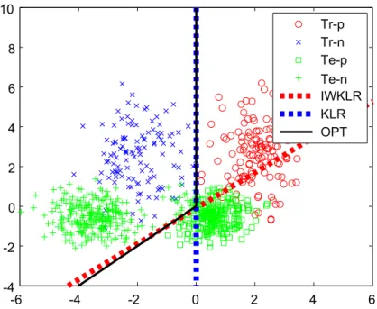
where OctoMag is the waveplayer and the SID system is the kernel- based speaker identification module. Each LED lights when the corre- sponding speaker is speaking. . . 26 4.1 Decision boundaries obtained by IWKLR+IWCV and KLR+CV (red
and blue dashed lines) and the optimal decision boundary (black solid line). ‘◦’ and ‘×’ are positive and negative training samples, while ‘¤’ and ‘+’ are positive and negative test samples. Note that the input- output test samples are not used in the training of KLR and the output test samples are not used in the training of IWKLR—they are plotted in the figure for illustration purposes. . . 37 5.1 Samples and contour plots of the true importance function, the esti-
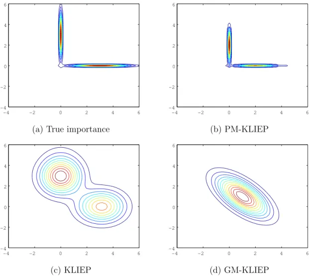
mated importance function by KLIEP, and an estimated importance function by GM-KLIEP in the illustrative example. . . 53
5.2 NMSEs averaged over 100 trials (log scale) in the illustrative examples. 54 5.3 Contour plots of the true importance function, and the importance
functions estimated by KLIEP, GM-KLIEP, and PM-KLIEP for the
illustrative example. . . 55
6.1 Recording Environment in anechoic chamber. . . 68
6.2 Noise reduction rate as a function of FDICA iteration for the two point source case in an anechoic chamber. The DOA of true sources are shown in the bracket (θ1, θ2). . . 69
6.3 Recording Environment in reverberant room. . . 70
6.4 Noise reduction rate as a function of FDICA iteration for the two point source case in a reverberant room. The DOA of true sources are shown in the bracket (θ1, θ2). . . 71
6.5 Recording Environment in diffuse interfering noise case. . . 72
6.6 Source separation result in interfering diffuse source case. . . 72
6.7 Source separation results in varying environmental conditions. . . 73
CHAPTER 1
INTRODUCTION
This dissertation is devoted to developing a useful speaker identification system for humanoid robots. In this chapter, we state the motivation and objective of our work.
1.1 Four issues in Speaker Identification for hu-
manoid robots
The speaker identification is one of the key technologies for person identification in humanoid robots. Especially, when the face information is not available, the speaker identification is the only way to identify person. Therefore, to improve the speaker identification performance is an important issue.
There are four major issues in speaker identification for humanoid robots. First, the humanoid robots should identify the speaker in real-time with high identification rates. Second, since the speech features vary over time due to session dependent variation, the recording environment change, and physical conditions/emotions, the robust speaker identification system under the feature changes is required. Third, the humanoid robots should automatically add the speakers in dictionary, when the un- known speaker talks to it. Forth, since humanoid robots move throughout the world, the surrounding environment, source positions, and source mixtures are constantly changing.
To cope with these issues, we address the following topics in this dissertation:
1. Kernel based real-time speaker identification with acceleration of Mean Opera- tor Sequence Kernel Computation
2. Semi-supervised Speaker Identification under Covariate Shift
3. Direct Importance Estimation with Gaussian Mixture Models and Probabilistic Principal Component Analyzers
4. Noise Adaptive Optimization of Matrix Initialization
In what follows, we present a brief introduction to each of these topics.
1.2 Kernel based real-time speaker identification
with Acceleration of Mean Operator Sequence
Kernel Computation
The humanoid robots should identify the speaker in real-time with high identifica- tion rates. In these days, the kernel methods such as the support vector machine (SVM) and kernel logistic regression (KLR) are popular for speaker identification tasks, and the kernel based system outperforms the conventional Gaussian Mixture Model (GMM) based system. However, the kernel based speaker identification sys- tem is originally expensive than GMM based speaker identification system, thus, the current version of kernel based speaker identification system is not suited for imple- menting on the humanoid robot. In addition, the kernel based speaker identification system usually uses the vectorial data, even though the sequential data is useful.
To cope with sequential speech data, a sequence kernel has been introduced for speaker identification [2], which utilizes a sequence of frame-level features for captur- ing long-term structure in phones, syllables, words, and the whole utterances. This sequence kernel is also called the Generalized Linear Discriminant Sequence (GLDS) kernel. While the GLDS kernel produced rather good performance in practice, it is not computationally efficient when the dimension of the feature space is very large;
this is because the GLDS kernel explicitly computes the projection of sequence sam- ples in the feature space. Due to this explicit computation, the GLDS kernel only allows us to employ finite-dimensional feature spaces such as the polynomial repro- ducing kernel Hilbert space (RHKS); infinite-dimensional feature spaces such as the Gaussian RKHS are not allowed to use.
To overcome this limitation, mean operator sequence kernel was introduced [1]. The mean operator sequence kernel measures similarity between two sequences by implicitly computing the inner product between the means of the sequences in the feature space. Therefore, it can deal with infinite-dimensional feature spaces. The mean operator sequence kernel based speaker verification system was shown to sig- nificantly outperform other methods such as GMM and SVM with finite-dimensional kernels.
However, the mean operator sequence kernel still has a weakness. The mean op- erator sequence kernel is often computationally more efficient than the GLDS kernel, but the mean operator sequence kernel is still computationally intensive; it requires N N′ vectorial kernel computations for measuring the similarity between sequential data of length N and N′.
The goal of this dissertation is to overcome this problem and develop a com- putationally efficient alternative to the original mean operator sequence kernel for real-time speaker identification system. Our basic idea is to approximate the mean operator sequence kernel using k-means algorithm. Then, we formulate the problem of approximating the sequence kernel as the problem of obtaining a pre-image in an RKHS [3], where pre-image xb is the vector in input space which corresponds to the vector in feature space.
1.3 Semi-supervised Speaker Identification under
Covariate Shift
In conventional methods, it is popular to assume that training and test speech data follow the same probability distribution. However, since the speech features vary over time due to session dependent variation, the recording environment change, and physical conditions/emotions, the training and test distributions are not necessarily the same in practice. In addition, the influence of the session dependent variation of voice quality in speaker identification problems has been investigated and the identi- fication performance was shown to decrease significantly over 3 months—the major cause for the performance degradation was the voice source characteristic variations [4].
To alleviate the influence of session dependent variation, it is popular to use sev- eral sessions of speaker utterance samples [5, 6] or to use cepstral mean normalization (CMN) [7]. However, gathering several sessions of speaker utterance data and as- signing the speaker ID to the collected data are expensive both in time and cost and therefore not realistic in practice. Moreover, it is not possible to perfectly remove the session dependent variation by CMN alone.
A practical setup for compensating the session dependent variation would be semi- supervised learning, where unlabeled samples are additionally given from the testing environment. In semi-supervised learning, it is required that the training and test distributions are related in some sense; otherwise we may not be able to learn any- thing about the test distribution from the training samples. A common modeling is called covariate shift, where the input distributions are different in the training and test phases but the conditional distribution of labels remains unchanged. In many real-world applications such as robot control [8, 9], bioinformatics [10, 11], spam fil- tering [12], natural language processing [13], brain-computer interfacing [14, 15], and
econometrics [16], the covariate shift model has been shown to be useful. Covari- ate shift is also naturally induced in selective sampling or active learning scenarios [17, 18, 19, 20, 21]. For this reason, learning under covariate shift is receiving a great deal of attention these days in the machine learning community [22].
In this dissertation, we formulate the semi-supervised speaker identification prob- lem in the covariate shift framework and propose a method that can cope with voice quality variants. Under covariate shift, standard maximum likelihood estimation is no longer consistent. The influence of covariate shift can be asymptotically canceled by weighting the log-likelihood terms according to the importance[23]:
w(X) = pte(X) ptr(X),
where pte(X) and ptr(X) are test and training input densities. We apply this weight- ing idea in KLR. The importance weight w(X) is unknown in practice and needs to be estimated from data. For weight estimation, we utilize the Kullback-Leibler importance estimation procedure (KLIEP) since it is equipped with a built-in model selection procedure [24]. The (regularized) kernel logistic regression model contain two tuning parameters: the kernel width and the regularization parameter. Usually those tuning parameters are optimized based on cross validation (CV). However, CV is no longer unbiased due to covariate shift and therefore is not reliable as a model selection method. To cope with this problem, we use importance weighted CV [15] for unbiased model selection. The validity of our approach is experimentally shown through text-independent speaker identification simulations.
1.4 Direct Importance Estimation using Gaussian
Mixture Models and Probabilistic Principal Com-
ponent Analysis
Humanoid robots are desired to automatically add the unknown speakers into dic- tionary, and it can be formulated as the outlier detection problem (i.e., outlier can
be the unknown speakers). Since the outlier detection problem can be solved via the log likelihood between the unknown speaker and the speakers in the dictionary, to improve the estimation accuracy of log likelihood is an important issue to for outlier detection problems.
Recently, the problem of estimating the ratio of two probability density functions (a.k.a. the importance or likelihood ratio) has received a great deal of attention since it can be used for various data processing purposes. Covariate shift adaptation would be a typical example [22]. Covariate shift is a situation in supervised learning where the training and test input distributions are different while the conditional distribution of output remains unchanged [23]. Another example in which the importance is useful is outlier detection [25]. The outlier detection task addressed in that paper is to identify irregular samples (i.e., outliers) in an evaluation dataset based on a model dataset that only contains regular samples (i.e., inliers). If the density ratio of two datasets is considered, the importance values for regular samples are close to one, while those for outliers tend to be significantly deviated from one. Thus the values of the importance could be used as an index of the degree of outlyingness. A similar idea can also be applied to change detection in time series [26].
A naive approach to approximating the importance function is to estimate train- ing and test probability densities separately and then take the ratio of the estimated densities. However, density estimation itself is a difficult problem and taking the ratio of estimated densities can magnify the estimation error. In order to avoid den- sity estimation, a semi-parametric approach called the Kullback-Leibler Importance Estimation Procedure (KLIEP) was proposed [27]. KLIEP does not involve density estimation but directly models the importance function. The parameters in the im- portance model is learned so that the Kullback-Leibler divergence from the true test distribution to the estimated test distribution is minimized without going through density estimation. KLIEP was shown to be useful in covariate shift adaptation [27]
and outlier detection [25]. A typical implementation of KLIEP employs a spher- ical Gaussian kernel model and the Gaussian width is chosen by cross validation. This means that when the true importance function is correlated, the performance of KLIEP is expected to be degraded.
To cope with this problem, we propose to use a Gaussian mixture model (GMM) in the KLIEP algorithm and learn the covariance matrix of the Gaussian compo- nents at the same time. This will allow us to learn the importance function more adaptively even when the true importance function contains high correlation. We develop an expectation-maximization procedure for learning the parameters in the Gaussian mixture model. The effectiveness of the proposed method—which we call the Gaussian mixture KLIEP (GM-KLIEP)—is shown through experiments.
In addition, since we need to estimate the inverse of covariance matrices for GM- KLIEP, it tends to be unstable when the rank-deficient input vectors are observed. To deal with the rank deficient data, it is popular to use the dimensionality reduction method such as principal component analysis (PCA) as a pre-processing tool. Thus, in this dissertation, we propose the mixture of probabilistic PCA model based impor- tance estimation, and we call the method as PPCA mixture KLIEP (PM-KLIEP).
1.5 Noise Adaptive Optimization of Matrix Ini-
tialization
In practice, the speech overlaps are frequently occurred during conversation, and it causes the serious degradation of speaker identification performance in humanoid robots. Thus, the source separation technique is preferred to use as the pre-processing of speaker identification system to improve the speaker identification performance. Therefore, in this dissertation, we propose the source separation method to improve the speaker identification performance in humanoid robot.
Implementing real-time frequency domain independent component analy- sis(FDICA) [28, 29, 30] has recently received much attention from the audio industry, c.f. [31]. This is due to the many potential source separation applications (e.g. speech enhancement, speaker separation), and the recent technological advancements that enable the implementation of FDICA on humanoid robots. However, since the humanoid robots move throughout the world, the surrounding environment, source positions, and source mixtures are constantly changing. Thus, it is quite difficult to implement FDICA in humanoid robots for real-world usage.
Many effective approaches have been proposed for improving FDICA performance by exploiting: knowledge regarding room and sensor geometry [32], geometric infor- mation of sound sources [33, 34], and a sophisticated prior model of speech [35]. However, these approaches implicitly assume knowledge of the sound source geome- try, the source type (point source, diffuse source, etc.), and are valid only in a specific surrounding environmental condition. In addition, since the cost function of FDICA is non-convex in nature, FDICA is not guaranteed to converge to the optimal solu- tion, when the initial unmixing matrix is incorrectly chosen. Thus, unmixing matrix initialization is a key factor for humanoid robot implementation of FDICA.
A popular unmixing matrix initialization technique is the combination of delay- and-sum (DS) and null beamformers (NBF) [30, 36], which are known to be robust to the well-known FDICA permutation problem [30]. However, beamformer-based initialization heavily depends on the sound source geometry and the source mixture type. Thus, beamformer-based initialization itself is not suited for mobile usage, without a reasonable estimator of the source geometry and the source types.
In this paper, we propose a Noise Adaptive Optimization of Matrix Initialization Algorithm (NAOMI). We assume a two source separation problem, where a point source, e.g., speech signal, is placed in front of a two microphone array, while a
second interfering source should be separated and removed using FDICA. The inter- fering source is either another point source that is not located directly in front of the microphones (e.g., a speech signal that is not intended to be captured by the micro- phones) or a diffuse source (e.g., loud background music or airplane engine rumble). To estimate the type of interfering source, we first estimate its direction of arrival (DOA) at each frequency bin using covariance fitting [37], and then use the statistics of the estimated DOAs to classify the interfering source. The initial unmixing matrix is then selected based on the estimated source type. The effectiveness of the pro- posed method for speech de-noising is evaluated via a source separation simulations in anechoic and reverberant rooms.
1.6 Organization of this dissertation
This dissertation consists of seven chapters. In this section, we show the organization of this dissertation.
Chapter 2 formulates the speaker kernel based identification problem and review existing methods such as KLR and CV. Then, we propose kernel based real-time speaker identification with acceleration of mean operator sequence kernel computation in Chapter 3. Chapter 4 is devoted to the semi-supervised speaker identification under covariate shift framework for alleviating the session dependent variation. In Chapter 5, importance weighting techniques using GMM and PPCA are introduced. In Chapter 6, we introduce the noise adaptive optimization of matrix initialization for practical source separation problem. Finally, Chapter 7 contains the conclusions and a section about future work.
CHAPTER 2
KERNEL-BASED SPEAKER IDENTIFICATION
In this chapter, we formulate the kernel based speaker identification approach and its model selection.
2.1 Problem formulation
An utterance feature X pronounced by a speaker is expressed as a set of N mel- frequency cepstrum coefficient (MFCC) [38] vectors of d dimensions:
X = [x1, . . . , xN] ∈ Rd×N. (2.1) For training, we are given ntr labeled utterance samples:
Ztr = {Xi, yi}ni=1tr, (2.2) where yi ∈ {1, . . . , K} denotes the index of the speaker who pronounced Xi. The goal of speaker identification is to predict the speaker index of a test utterance sample X based on the training samples. We predict the speaker index c of the test sample X following the Bayes decision rule:
P (y = c|X) > P (y = i|X) ∀ i 6= c. (2.3) For approximating the class-posterior probability, we use the following parametric model p(y = c|X, V):
p(y = c|X, V) = PKexp fvc(X)
l=1exp fvl(X)
, (2.4)
where V = [v1, . . . , vK]⊤ ∈ RK×ntr is the parameter, ⊤ denotes the transpose, and fvl is a discriminant function corresponding to the speaker l. This model is known as the softmax function and widely used in multiclass logistic regression. We use the following kernel regression model as the discriminant function fvl [6]:
fvl(X) =
ntr
X
i=1
vl,iK(X, Xi) l = 1, . . . , K, (2.5) where vl = (vl,1, . . . , vl,ntr)⊤ ∈ Rntr are parameters corresponding the speaker l and K(X, X′) is a kernel function.
2.2 Feature Extraction
In speaker identification, it is common to extract a set of features from each speech signal, and we use the extracted feature for classification instead of the speech signals themselves. A good set of features should include discriminative information, and the feature set should be small enough to allow fast processing and robust.
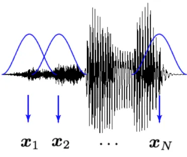
A speech signal can be assumed as a stationary stochastic process within small time intervals (20-30ms). From this fact, the major discriminative information be- tween speech signals appear in the frequency domain, and we usually use the sequence of short time spectral feature vectors which extracted from the speech signal. Figure 2.1 illustrates the extraction of a feature vector X = [x1, . . . , xN] from a speech sig- nal. A window function of fixed width such as Hamming window is used to extract a short-time segment of the speech signal in order to convert to the spectral feature vector. Then, the window function is shifted with 5-10 ms to the right for further extraction of feature vectors until the end of the speech signal is reached. Note that, since different speech signals have different durations, feature extraction with a fixed window shift leads to time series with different number of vectors.
Mel-frequency cepstral coefficients (MFCC) [38] are both popular feature extrac- tion methods. Often, the energy of the windowed speech signal is appended to the MFCC feature vectors. The total dimension of these feature vectors is usually 13.
Figure 2.1: Feature extraction from a speech signal.
We also use the delta and accelerationcoef f icients of the feature vectors for improving recognition performance. Delta coefficients (∆ MFCC) are the first order time derivatives of a feature vector sequence, and contain information on the rate of change of the vectors in the sequence. Similarly, acceleration coefficients (∆∆ MFCC) are the approximations to the second order time derivatives, and contain information on the rate of the rate of change. We usually concatenate the MFCC coefficients, ∆ MFCC, and ∆∆ MFCC, and we use the vector for speaker identification.
2.3 Kernel Logistic Regression
Logistic regression is a one of the popular statistical method for estimating the con- ditional probability distribution p(y|X) of a class label y ∈ Y given an observation X ∈ X . Classification is accomplished by selecting the class label ˆy given the largest conditional probability:
ˆ
y = arg max
y∈Y p(y|X). (2.6)
For approximating the class-posterior probability, we use the following parametric model p(y = c|X, V):
p(y = c|X, V) = PKexp fvc(X)
l=1exp fvl(X)
, (2.7)
where V = [v1, . . . , vK]⊤∈ RK×ntr is the parameter,⊤ denotes the transpose, and fvl is a discriminant function corresponding to the class y = l. This function is known as sof tmax function. Kernel logistic regression (KLR) is a kernelized variant of logistic regression. In KLR, we map the input vector to a high-dimensional space (feature space) and solve the logistic regression problem in the feature space; the similarity in feature space can be implicitly computed via the kernel trick. The kernel trick allows one to non-linearize a linear algorithm without sacrificing computational simplicity of the linear algorithm. Below, we briefly review KLR following the papers [39, 40].
We employ maximum likelihood estimation for learning the parameter V. The negative log-likelihood function Pδlog(V; Ztr) for the kernel logistic regression model is given by
Pδlog(V; Ztr) = −
ntr
X
i=1
log P (yi|Xi, V) + δ
2trace(VKV
⊤), (2.8)
where trace(VKV⊤) is a regularizer to avoid overfitting, δ is the regularization pa- rameter that controls strength of regularization, and K = [K(Xi, Xj)]ni,j=1tr is the kernel Gram matrix. The negative log-likelihood function is convex and the unique mini- mizer can be obtained by, e.g., the Newton method. In the Newton method, the parameter matrix V is updated iteratively as
V ← V − ²∆V, (2.9)
where ² is the step size and ∆V is defined as
vec∆V = [∇2Pδlog(V; Z)]−1vec∇Pδlog(V; Z). (2.10)
‘vec’ denotes the vectorization operator, ∇Pδlog(V; Z) is the gradient of Eq.(2.8) with respect to V, and ∇2Pδlog(V; Z) is the Hessian of Eq.(2.8) with respect to V. The
gradient and Hessian are given as
∇Pδlog(V; Z) = (P(V) − Y + δV)K, (2.11)
∇2Pδlog(V; Z) =
ntr
X
i=1
(diag(p(Xi)) − p(Xi)p(Xi)⊤) ⊗ k(Xi)k(Xi)⊤
+(K⊤⊗ I), (2.12)
where
P(V) = [p(X1), . . . , p(Xntr)] ∈ R
K×ntr (2.13)
is a matrix whose n-th column is a vector of the class-posterior probabilities p(Xn), p(X) = [p(y = 1|X, V), . . . , p(y = K|X, V)]⊤ ∈ RK (2.14) denotes the class-posterior probabilities for all classes given X,
Y = [ey1, . . . , eyN] ∈ RK×ntr, (2.15) whose n-th column eyn is a unit vector with all zeros except for element yn being 1, diag(a, . . . , b) denotes the diagonal matrix with diagonal elements a, . . . , b,
k(X) = [K(X, X1), . . . , K(X, Xntr)]⊤ ∈ Rntr (2.16) is a vector whose elements are given by the mean operator sequence kernel, ⊗ denotes the Kronecker product, and I denotes the identity matrix.
In order to estimate the update matrix ∆V, the inverse of the Hessian needs to be computed at every iteration. This is computationally expensive so we approximate
∆V by the conjugate gradient method; an approximation d∆V can be estimated by solving the following linear equation [39, 40]:
∇2Pδlog(V; Z)vecd∆V = vec∇Pδlog(V; Z). (2.17) Substituting Eqs.(2.11) and (2.12) into Eq.(2.17) and using the transformation
vec(ABC) = (C⊤⊗ A)vec(B), (2.18)
we have
ntr
X
i=1
(diag(p(Xi)) − p(Xi)p(Xi)⊤)d∆Vk(Xi)k(Xi)⊤ = (P(V) − Y + δV)K.
(2.19) 1. Initialize: Start with an initial matrix ∆Vi0 and compute the matrices R0 and Q0:
R0 = P(Vi) − Y + δV
− XN
j=1
ejk(Xi)∆V0i(diag(p(Xi)) − p(Xi)p(Xi)⊤) − δ∆Vi0, (2.20) Q0 = k(Xi)e⊤j R0(diag(p(Xi)) − p(Xi)p(Xi)⊤) − R0. (2.21) 2. Iterate: Generate a sequence (∆Vi1, ∆V2i, . . .) according to
αk = k(Xi)e
⊤j R0(diag(p(Xi)) − p(Xi)p(Xi)⊤) + Rk
ejk(Xi)⊤Qk(diag(p(Xi)) − p(Xi)p(Xi)⊤) + Qk
, (2.22)
∆Vk+1i = ∆ikVik+ αkRk, (2.23)
Rk+1 = P(Vi) − Y + δV
− XN
j=1
ekk(Xi)∆Vk+1i (diag(p(Xi)) − p(Xi)p(Xi)⊤) − δ∆Vik+1, (2.24)
βk = k(Xi)e
⊤j Rk+1(diag(p(Xi)) − p(Xi)p(Xi)⊤) + Rk+1
k(Xi)e⊤j Rk(diag(p(Xi)) − p(Xi)p(Xi)⊤) + Rk
, (2.25)
∆Vk+1i = ∆ikVik+ αkRk, (2.26)
Qk+1 = k(Xi)e⊤j Rk+1(diag(p(Xi)) − p(Xi)p(Xi)⊤) − Rk+1. (2.27)
2.4 Mean Operator Sequence Kernel
The performance of KLR depends on the choice of the kernel function. A popular choice for speaker identification is the mean operator sequence kernel, which is defined as follows [1]:
K(X, X′) = 1 N
XN p=1
φ(xp)⊤ 1 N′
N′
X
p′=1
φ(x′p′),
= 1
N N′ XN
p=1 N′
X
p′=1
k(xp, x′p′)
where
X = [x1, . . . , xN] ∈ Rd×N, X′ = [x′1, . . . , x′N′] ∈ Rd×N′,
are sequences of d-dimensional features of length N and N′ and
k(x, x′) = φ(x)⊤φ(x′)
is a ‘base’ vectorial kernel function.
In this dissertation, we use the Gaussian kernel for ‘base’ vectorial kernel function:
k(x, x′) = exp
µ−kx − x′k2 2σ2
. (2.28)
2.5 Model selection in Kernel Logistic Regression
The above KLR method includes two tuning parameters: the Gaussian width σ and the regularization parameter δ. KLR is shown to be consistent, i.e., the learned parameter converges to the optimal value as the number of training samples tends to be infinity:
N →∞lim V = Vb
∗,
where bV is the parameter learned by KLR and V∗ is the optimal parameter that minimizes the expected prediction error for test samples:
V∗ = argmin
V
ZZ
I(y =by(X | V))p(y | X)p(X)dydX.
b
y(X | V) is an estimate of speaker of an utterance feature X for parameter V. Also, when p(X) and p(y | X) are common in the training and test phases, cross-validation (CV) is (almost) unbiased [3]:
EZtr
hRbZCVtr − RZtri ≈ 0,
where EZtr is the expectation over the training set Ztr and RZtr is the expected prediction error defined by
RZtr = ZZ
I(y =by(X; Ztr))p(y | X)p(X)dydX.
b
y(X; Ztr) is a learned function from the training set Ztr.
One of the popular approaches to model selection is k-fold cross validation (kCV). Let us divide the training set Ztr = {(Xi, yi)}ni=1tr into k disjoint non-empty subsets {Zitr}ki=1. Let byZtr
j (X) be an estimate of a speaker of a test utterance sample X obtained from {Zitr}i6=j (i.e., without Zjtr). Then the score is given by
RbZkCVtr = 1 k
Xk j=1
1
|Zjtr| X
(X,y)∈Zjtr
I(y =ybZtr
j (X)), (2.29)
where |Zjtr| is the number of samples in the subset Zjtr and I(·) denotes the indicator function.
CHAPTER 3
KERNEL BASED REAL-TIME SPEAKER
IDENTIFICATION WITH ACCELERATING
SEQUENCE KERNEL COMPUTATION
This chapter is devoted to developing a kernel based real-time speaker identification.
3.1 Introduction
Kernel methods such as the support vector machine (SVM) [41] and kernel logistic regression (KLR) [42] are successful approaches in speaker identification, given that the kernel functions are designed appropriately. Recently, a mean operator sequence kernel (MOSK) has been introduced for speaker identification [1], which utilizes a se- quence of frame-level features for capturing long-term structure in phones, syllables, words, and entire utterances. MOSK measures the similarity between two sequences by computing the inner product between the means of the sequences implicitly in the feature space. The MOSK based speaker verification system was shown to signifi- cantly outperform other methods such as the Gaussian mixture model (GMM) and the SVM with finite-dimensional kernels.
Although MOSK performs well in the speaker verification task, its computational complexity limits its use in applications where real time processing is required. Specif- ically, MOSK requires N N′ vector kernel computations for measuring the similarity
between two data sequences of length N and N′, respectively. The goal of this pa- per is to develop a computationally efficient alternative to the MOSK for real time speaker identification. The first step in our approach is to approximate the MOSK using k-means clustering. Then, we formulate the problem of approximating the se- quence kernel as the problem of obtaining a pre-image in a reproducing kernel Hilbert space (RKHS) [41]. A pre-image is a vector in the input space mapped to the target feature vector in the RKHS.
The practical effectiveness of the proposed method is investigated in text- independent speaker identification experiments with 10 male speakers. Results demonstrate that the proposed method provides significant reduction in computation time while speaker identification accuracy is only moderately degraded. Furthermore, using the pre-image approximation we develop a real-time speaker identification sys- tem using Virtual Studio Technology (VST).
3.2 Problem Formulation
In this section, we formulate the speaker identification problem based on the kernel logistic regression (KLR) model.
3.2.1 Kernel-based Text-independent Speaker Identification
An utterance sample X pronounced by a speaker is expressed as a set of N mel- frequency cepstrum coefficient (MFCC) [38] vectors of dimension d:
X = [x1, . . . , xN] ∈ Rd×N.
For training, we are given n labeled utterance samples:
Z = {(Xi, yi)}ni=1,
where yi ∈ {1, . . . , K} denotes the index of the speaker who pronounced Xi. The goal of speaker identification is to predict the speaker index of a test utterance sample X
based on the training samples. We predict the speaker index c of the test sample X following Bayes decision rule:
maxc p(y = c | X).
For approximating the class-posterior probability, we use
p(y = c | X; V) = PKexp fvc(X)
l=1exp fvl(X)
,
where V = [v1, . . . , vK]⊤ ∈ RK×nis the parameter,⊤ denotes the transpose, and fvl is a discriminant function corresponding to speaker l. This form is known as the softmax function and widely used in multiclass logistic regression. We use the following kernel regression model as the discriminant function fvl:
fvl(X) = Xn
i=1
vl,iK(X, Xi) l = 1, . . . , K,
where vl = (vl,1, . . . , vl,n)⊤ ∈ Rn are parameters corresponding to speaker l and K(X, X′) is a kernel function.
We employ maximum likelihood estimation for learning the parameter V. The negative log-likelihood function Plog(V; Z) for the kernel logistic regression model is given by
Plog(V; Z) = − Xn
i=1
log P (yi| Xi; V),
where K = [K(Xi, Xj)]ni,j=1is the kernel Gram matrix. Plog(V; Z) is a convex function with respect to V and therefore its unique minimizer can be obtained using, e.g., the Newton method [39].
3.2.2 Mean Operator Sequence Kernel [1]
The performance of KLR depends on the choice of the kernel function. In this chapter, we use the mean operator sequence kernel (MOSK) [1] as the kernel function since
it allows us to handle feature sequences of different length. For sequences of d- dimensional feature vectors of length N and N′,
X = [x1, . . . , xN] ∈ Rd×N, X′ = [x′1, . . . , x′N′] ∈ Rd×N′, MOSK is defined as
K(X, X′) = 1 N
XN p=1
φ(xp)⊤ 1 N′
N′
X
p′=1
φ(x′p′),
= 1
N N′ XN
p=1 N′
X
p′=1
k(xp, x′p′),
where
k(x, x′) = φ(x)⊤φ(x′) is a ‘base’ vector kernel function.
MOSK requires N N′ vector kernel computations for calculating the similarity between utterances X and X′. Therefore, the MOSK computation is not suited for real-time application when N N′ is very large.
3.3 Approximation of MOSK
In this section, we provide an approximation method of the MOSK computation. Below, we focus on the Gaussian kernel as the base kernel function:
k(x, x′) = exp µ
−kx − x
′k2
2σ2
¶ .
3.3.1 Approximating Mean Operator Sequence Kernel by Parts
For D ¿ N , let us divide the samples {x1, . . . , xN} into D clusters {C1, . . . , CD} such that
Ci∩ Cj = ∅ for i 6= j, C1∪ · · · ∪ CD = {x1, . . . , xN}.
We may use the k-means clustering algorithm for this purpose. Then, N1 PNp=1φ(xp) can be expressed as
1 N
XN p=1
φ(xp) = 1 N
(X
x∈C1
φ(x) + · · · + X
x∈CD
φ(x) )
.
= π1 N1
X
x∈C1
φ(x) + · · · + πD ND
X
x∈CD
φ(x), (3.1)
where Ni is the number of samples in cluster Ci and πi = Ni/N . If we can approximate the mean N1
i
P
x∈Ciφ(x) by a single point φ(mi), the com- putational cost of the mean in the feature space is reduced from O(N ) to O(D). To obtain a good approximation point mi, we minimize the following criterion:
Ji(mi) = kφ(mi) − 1 Ni
X
x∈Ci
φ(x)k2.
This is often called the pre-image problem in the context of kernel methods [41]. For the Gaussian kernel, the above criterion can be written as
Ji(mi) = 1 − 2 Ni
X
x∈Ci
k(mi, x) + 1 Ni2
X
x,x′∈Ci
k(x, x′), (3.2) where we used
k(mi, mi) = exp µ
−kmi− mik
2
2σ2
= 1. Taking the derivative of Eq.(3.2) with respect to m, we have
∂Ji(mi)
∂mi
= ∂
∂mi
"
− 2 Ni
X
x∈Ci
exp µ
−kmi − xk
2
2σ2
¶#
= 1 σ2Ni
X
x∈Ci
exp µ
−kmi− xk
2
2σ2
(mi− x). (3.3)
Equating Eq.(3.3) to zero, we have
c mi =
P
x∈Ciexp
³−km2σi−xk2 2
´ x P
x′∈Ciexp³−km2σi−x2′k2
´ . (3.4)
We use Eq.(3.4) as a re-estimation formula, i.e., cmi is updated by Eq.(3.4) with mi
in the right-hand side replaced by the current estimate cmi and this is repeated until convergence.
Then Eq.(3.1) yields 1 N
XN p=1
φ(xp) ≈ XD
i=1
πiφ(cmi). (3.5)
Based on Eq.(3.5), MOSK can be approximated by K(X, X′) ≈
XD i=1
πiφ(cmi)⊤
D′
X
i′=1
π′i′φ(cmi′)
= XD
i=1 D′
X
i′=1
πiπi′′k(mci,mci′). (3.6)
Following the k-means clustering algorithm, we call the proposed method the k-means operator sequence kernel (k-MOSK). The number of vectorial kernel computations in the original MOSK is N N′, while that in k-MOSK is DD′. Thus k-MOSK would be computationally much more efficient than MOSK given that D and D′ are much smaller than N and N′. It is clear that k-MOSK satisfies positive definiteness; thus it is a valid kernel function.
The computation of the k-means clustering algorithm for every utterance in the test phase is expensive. So we compute the kernel between a training sample X and a test sample X′ = {x′1, . . . , x′N′} as
K(X, X′) = 1 N′
XD i=1
N′
X
p=1
πik(cmi, x′p). (3.7)
3.4 Experiments
In this section, we compare the performance of MOSK and k-MOSK with different numbers of clusters D in a speaker identification task.
3.4.1 System and Data Acquisition
The data for training and testing were collected from 10 male speakers, where each speaker uttered several different words as listed in Table 3.1.
The duration of an utterance for each training sentence was approximately four seconds. Thus, the total duration of utterances over three training sentences was
Table 3.1: Training sentences and test words (in Japanese, written using the Hepburn system of Romanization).
Contents
Training 1. seno takasawa hyakunanajusseNchi sentences: hodode mega ookiku yaya futotteiru
2. oogoeo dashisugite kasuregoeni natte shimau
3. tashizaN hikizaNwa dekinakutemo eha kakeru
Testing 1. mouichido words: 2. torikaeshi
3. teisei 4. horyuu 5. shoukai
approximately 12 seconds per speaker. For testing purposes, we use utterances of 5 words recorded in three sessions over six months with no time overlap to the training session. Thus the total number of test words was 150 (10 speakers × 5 words × 3 sessions).
A feature vector of 26 dimensions, consisting of 12 MFCCs, normalized log en- ergy, and their first derivatives, is derived once every 10ms over a 25.6ms Hamming- windowed speech segment. We divide each training utterance into 300ms disjoint segments, each of which corresponds to a set of features of size 26 × 30. On the other hand, for testing, we use the whole utterance of each word consisting of approximately 1000ms duration for computing MOSK and k-MOSK since each word is treated as a single test sample.
3.4.2 Results
We evaluate the proposed k-MOSK with the several different numbers of clusters D. The Gaussian width σ in the base Gaussian kernel is chosen from
{8, 10, 12, 14, 16}
5 10 15 20 25 30 0.5
0.6 0.7 0.8 0.9 1
Number of Clusters
Identification Rates
Mosk k-Mosk
Figure 3.1: Speaker identification rates obtained using 30, 15, 10, and 5 clusters, with selected kernel widths of 12, 14, 14, and 16, respectively.
by 10-fold cross-validation (CV). In our preliminary experiments, we observed that the 10-fold CV scores tend to be heavily affected by the random split of the training samples. We conjecture that this is due to non-i.i.d. nature of the MFCC features, which is different from the theoretical assumptions of CV. In order to obtain reliable experimental results, we repeat the CV procedure 50 times with different random data splits and use the average score for model selection.
Figure 3.1 depicts the speaker identification rates for the test words using MOSK and k-MOSK with different numbers of clusters D. In Figure 3.2, we plot the compu- tation time of MOSK and k-MOSK in training and testing using a standard personal computer with a Quad Core 2.0GHz processor and 2GB memory. The computation time for MOSK is normalized to one. These results demonstrate that k-MOSK is computationally more efficient than the original MOSK with mild degradation in identification accuracy.
Based on k-MOSK, we have developed a real-time kernel-based speaker identifi- cation system using a Virtual Studio Technology (VST) plugin (see Figure 3.3). A demo movie is available at http://dsp.syuriken.jp/demo/sid.html.
5 10 15 20 25 30 0.4
0.6 0.8 1
Number of Clusters
Normalized Time
Train Test
Figure 3.2: The normalized computation time of MOSK and k-MOSK in training and testing using a standard personal computer with Quad Core 2.0GHz processor and 2GB memory.
Figure 3.3: Five-speaker identification system implemented with the VST plugin, where OctoMag is the waveplayer and the SID system is the kernel-based speaker identification module. Each LED lights when the corresponding speaker is speaking.