Detecting misfits of the ETAS for seismicity anomalies
Takao Kumazawa
Doctor of Philosophy
Department of Statistical Science
School of Multidisciplinary Sciences
The Graduate University for Advanced Studies
2011
Table of Contents
Ch1. Introduction
1-1. Why in search of anomalies in seismicity --- 3
1-2. Coulomb stress changes --- 4
1-3. Point Process --- 4
1-4. ETAS model --- 6
Ch.2: Change-point Method 2-1. Introduction to change-point method --- 7
2-2. The degree of freedom for a change-point --- 8
2-3. Error bound of the change-point estimate ---11
2-4. Change-point in seismicity ---11
2-5. Application to the 2008 Iwate-Miyagi Nairiku, Japan, earthquake --- 12
2-6. Discussion of change-point analysis --- 46
2-7. Conclusion so far --- 50
2-8. Some afterthoughts (with respect to Tohoku earthquake of M9.0) --- 51
Ch.3 Misfit functions 3-1. Introduction to misfit functions --- 52
3-2. Misfit functions --- 53
3-3. Applications to the earthquakes of selected regions --- 57
3-4. Data with swarms --- 58
3-5. Seismic anomalies before M9.0 Tohoku earthquake --- 71
3-6. Seismicity triggered by M9.0 Tohoku-Oki earthquake --- 84
3-7. Examination by Simulation --- 104
3-8. Conclusions and discussions --- 107
Ch.4 Conclusion --- 109
Acknowledgements--- 109
Inferences --- 111
3
Ch1. Introduction
1,1 Why in search of anomalies in seismicity
It is a challenging task to predict a coming large earthquake. It is still fresh in our memory that basically none of scholars had ever assumed such a huge earthquake as M9.0 Tohoku-Oki earthquake would have occurred in that region. Besides the complex nature of crustal dynamics that underlies seismogenic faulting, one of the difficulties, in the statistical point of view, of the prediction lies in the limited number of previous precedents. The typical recurrence intervals of major active faults in Japan, for example, ranges from a few to several thousand years [Nomura et al. 2011], some of which earthquakes previously occurred before the history. Unlike weather forecasting, such limitation in the consultable precedents put us into a difficult situation that, if try to forecast an earthquake from seismicity data alone, we are in desperate need of carefully studying every unusual phenomenon which deviates from what we consider as normal. Putting this in other words, studying anomalies in seismicity and accumulating the knowledge from it is the key to understand what has been and will be going on in the ground beneath. There are possibly as many sources of anomalies as one can think of, but we may roughly summarize their qualities into two categories; disturbances from outside, and from inside. The external causes would include volcanic activities, which contaminate data with earthquakes driven by the mechanism different from the normal seismicity of the focal region. Another example is shear stress changes transferred from nearby faulting dynamics. We will explore the latter cause further more in the following section of 1-2. The internal causes would include slow slip events inside the fault of our concern.
In the remainder of this chapter, we review the ETAS model and its treatments. The ETAS model is intensively used in this thesis, hence the good understanding of the model is indispensable. In chapter 2, we extend the ETAS model to have change-points, across which some of the parameters in the ETAS model change. We use this method to examine if there were any anomalies in the seismicity before the 2008 Iwate-Miyagi earthquake of M7.0. In chapter 3, we introduce misfit functions of the ETAS model, and apply them to the cases in which more complicated anomalies are possibly expected.
3
1-2. Coulomb stress changes
There might be considerable reasons to have regional changes in seismicity. We will investigate the relation between regional changes of seismicity and stress that are caused by abrupt or slow slips in a local region on a fault. Reasenberg and Simpson [1992] and Toda and Stein [2003] report that changes in seismicity rate correlate with the calculated increment of the Coulomb failure stress:
ΔCFS = Δ(shear stress) − μ’Δ(normal stress)
where μ’ represents the apparent friction coefficient, and positive normal stress indicates compression. In the paper, we set μ’ = 0.4 to minimize the effect of
uncertainties and to make ΔCFS patterns stable with respect to changes in μ’ [King et al., 1994], unless receiver faults are very close to the ruptured fault. The change of Coulomb failure stress in an elastic half-space is calculated by assuming a shear modulus of 3.2 × 10¹¹dyn cm−2 and a Poisson ratio of 0.25 [Okada, 1992]. Positive values of ΔCFS promote failure and negative ones inhibit failure. In particular, Simpson and Reasenberg [1994] and Harris [1998] refer to a region of negative ΔCFS values as
‘stress shadow.’ Some retrospective case studies [Ogata et al., 2003; Ogata, 2005, 2006a, 2007, 2010] support the assertion that the stress shadow inhibits normal decay of aftershock activity, i.e., the activity becomes significantly lower than the decay rate predicted by the model.
The rate/state friction law of Dieterich [1994] provides the quantitative physical basis of the shadowing and activation of seismicity. For example, it implies that decreasing rate of aftershock occurrence in an aftershock area can be locally accelerated by either the negative ΔCFS due to abrupt slip [Harris and Simpson, 1998; Toda and Stein, 2003] on a fault or a transient stressing rate decrease due to a slow slip on a fault [Dieterich et al., 2000; Ogata and Toda, 2010; Ogata, 2010]. Numerical simulations based on the
rate/state friction also demonstrated the detectable changes in seismicity rate can be reproduced by loading rate changes associated with a slow slip [Ogata and Toda, 2010; Ogata, 2010].
1,3 Point Process
The seismic activity tends to cluster in its own nature, due mainly to the following
5
aftershocks. The modeling of such an triggering effect needs to capture the clustering nature, and accordingly various attempts have been tried. The majority of them use (homogeneous) Poisson process to describe the primary events, and let each of the event produce a number of offsprings, or aftershocks. We now introduce briefly the idea and treatments of point process in general. A point process [Daley and Vere-Jones, 2003] represents the probability of an event occurrence within a small time interval of length Δ, as
Pr{N(t,t)event history}
t . (1-1) Here
N(s,t) denotes the number of events in-between time s and t. The conditional intensity function
t then represents the occurrence rate of an event that depends on the history: the occurrence times and magnitudes of past events. The epidemic type aftershock sequence (ETAS) model [Ogata, 1988, 1989] is one of such models, and it has been widely used in the area of modeling seismic sequences. We will introduce the ETAS model in the next section 1-4. In the reminder of this chapter we first cover general treatment for point process analysis.Provided a sequence of occurrence times of earthquakes coupled with their magnitudes in an observed period
S, , the parameter setT
are estimated by maximizing the log-likelihood function [Daley and Vere-Jones, 2003]
ln L
ln
ti lnS
T {i:St
iT }
t , (1-2) where ti , represents the occurrence time of the i-th earthquake.We use maximum likelihood estimator (MLE)
to predict the future occurrence rateˆ
ˆ
t , t > T. Utsu and Ogata [1997] detail the computational aspects to obtain the MLE.To see how the estimated model performs, we use the integrated occurrence rate,
S t u dut
S ( )
, ˆ
ˆ
. (1-3)
This shows the estimated cumulative number of events over the period [S,t]. Plotting this together with the observed cumulative number of earthquakes N(S,t) makes its performance easily seen by the eye. See Ogata and Shimazaki [1984], Matsu'ura [1986], Ogata [1988, 1992, 1999a], Utsu et al. [1995] for examples. If we transform the
5
normal time t intoτso that
(S,t), then the sequence of event occurrence
t1,t1,,tN
is transformed one-to-one into
1,1,,N
. This transformed sequence follows the Poisson process with unit rate, namely, uniformly random distribution on
0, S,T
if Λis that of the true model. Thus when the estimated rate of earthquake occurrence
S,t
approximates well enough the real seismicity, it closely overlaps the observed cumulative counts
N[S,t] for t larger than T, in other words
S,t provides a reliable prediction. In the similar way the transformed sequence of data
ˆ1,ˆ1,,ˆN
distributes uniformly over the period
0,ˆ
S,T
if the estimation is good.1-4.ETAS model
The ETAS model, first introduced by Ogata [1986, 1988] has the following specific expression;
(t) Ki
t ti c
p{i:St
it}. (1-4)
The term
t ti c
p represents the empirical rule of modified Omori-Utsu formula for aftershock decay. This model treats the case in which an event (earthquake) i that occurring at time
ti triggers its offspring events, hence the seismicity rate at time t is given by the linear superposition of all aftershock effects in its past. The sum is taken for all events i occurred before time t. The constant μ wraps up all the factors of
occurrence rate that cannot be explained by aftershock effect of the past available data. The coefficient
Ki uses G-R law, i.e., it depends on its magnitude
Mi as well as the cut-off magnitude
Mz of the data set, in such a way that
Kj K0e(MiMz ). (1-5) The parameter set θ thus consists of five elements of
,K0,c,, p
. We have used“Statistical Analysis of Seismicity-updated version (SASeis2006)” [Ogata, 2006b] to calculate the MLE of θ, and to visualize model performances as well.
7
Ch.2: Change-point Method
2.1 Introduction to change-point method
At times it is reasonable to believe that one or more of a model’s parameters change at certain point in time. In such case treating those parameters independently before and after that point may give better results. Or, we can say the model is improved. Our concern of whether the seismicity changes after some time T0 in a given period [S, T] is a problem among such model selections, i.e. whether the model fitted separately before and after T0 then combined together, outperforms the model fitted throughout the period [S, T]. On comparing the performances between models, we consult the Akaike information criterion (AIC) [Akaike, 1973, 1974, 1977], described as
AIC 2max lnL()2k, (2-1)
with k being the number of parameters to be estimated. Under this criterion, the model with smaller value of AIC performs better. Our comparison here is made between the AIC12 for the combined model and AIC0 for the model fitted throughout the whole period. Precisely, we consider following
2 2 0 2
1 0 1 1
0 0
0
2 ) ,
; ( ln max 2
2 ) ,
; ( ln max 2
2 ) ,
; ( ln max 2
2 1
0
k T T L AIC
k T S L AIC
k T S L AIC
and
AIC12 AIC1AIC22q, (2-2)
where q represents the degree of freedom imposed on searching the time T0 based on the data over whole period, and each log likelihood
ln L(;A,B) is to be maximized over the parameter set using the data from the time period [A, B]. The minimum of AIC12
calculated throughout the target period [A, B] gives the MLE of the change point T0.
AIC12 being smaller than AIC0 marks the time T0 as the significant change-point, which means the seismicity pattern has significantly changed across the time T0. If T0 is determined independently of the data, in such a case when T0 is prefixed before the parameter estimation, then q is zero hence comparing AIC0 with AIC12 as the sum of
7
AIC1 and AIC2 alone will tell the significance of the prefixed change-point. Our treatment is otherwise and hence in need of quantifying q. In the next section we will discuss a heuristic evaluation procedure of the penalty q. In our applications to the Iwate-Miyagi earthquakes, we set T0 at every interval of events, then chose the one that minimize the AIC12, then compared it with the AIC without a change-point.
One may also be interested in the error range of the change-point. Although the standard theory for the MLE error estimate is not applicable to the change-point problem, we can provide confidence intervals in terms of the AIC differences. See section 2-3 for the detail.
2.2 The degree of freedom for a change-point
Assume that a model
H0is included in a model
H1that has k extra number of parameters. Then, the large sample theory implies that the likelihood ratio statistic
(-2)log ˆ
L 0 L ˆ 1 distributes according to
k2with degree of freedom k. The penalty term of the AIC is derived based on this property and has the following relationship
(-2)log ˆ
L 0 L ˆ 1 AIC(H0) AIC(H1) 2k . (2-3)However, the ordinary large sample theory cannot be applied to the change-point problem [Chernoff and Rubin, 1956]. Therefore, we apply a Monte-Carlo simulation for the likelihood ratio as follows. Simulate uniformly random points on the unit interval [0, 1] with a number N1 = N[0, 1] as the null hypothesis H0 (stationary Poisson process), and consider the alternative model H1 to be uniform distributed in respective separated intervals [0,T0] and [T0, 1] with any change-point T0 (piecewise stationary Poisson processes). Then we calculate the likelihood ratio of the form
1 1
0 1 1
1 0 1 0
0 ˆ 2max log log 1 2 log
log ˆ ) 2
(- 0 0 0 0
0 T N N
N N N
T N N N
L
L T T T T
T ,
(2-4) with Nt N[0,t]. To see the distribution of the values, we repeat the simulation 10,000 times. For example, the histogram in Fig. 2-01 shows the distribution of
9
ˆ ˆ
1 log) 2
(- L0 L1 with N = 1000, which removes one degree of freedom due to the fact that the alternative have the one more occurrence rate for the latter period. It turns out that, unlike the case of the ordinary likelihood ratio statistic, this distribution differs depending on the different number of N on the unit interval [0, 1], and the average of this distribution are given by the ratio of polynomials
3 2
3 2
0090963 10 .
10 0 95595 . 10 0 0900 . 5 1
045644 10 .
10 0 9376 . 10 3 325 . 15 1
) (
N N N
N N
N N
q (2-5)
This function is graphed in Fig. 2-02. It is a smoothly increasing concave function that approaches to around 6 with N increases. With the size of data set we dealt with, it ranges from 4 to 5. This Pade approximant in (2-5) is obtained by the least squares of the simulation experiments with the different numbers 10 ≤ N ≤ 2000. We note here that q(N) in Ogata [1992, 1999b] includes an error, and should be corrected as the above.
9
Figure 2-01. The distribution of
(-2)log ˆ
L 0 L ˆ 1 1 by simulation, with N=1,000. The red line shows their mean. The blue line shows twice the mean, that is, the AIC for the change-point.
Figure 2-02. A plot of Equation 2-5, with number of events N from 10 to 2000.
11 2-3. Error bound of the change-point estimate
Error bounds of the MLE are calculated by the normal distribution approximation of the likelihood function around the MLE. For example, see Aki [1965] for the b-value estimate of the magnitude frequency. However, this procedure cannot be applied to the change-point problem [e.g., Chernoff and Rubin, 1956]. Alternatively, we calculate them based on the theory from which the AIC is derived. Fundamentally, the AIC is the unbiased estimator of the logarithm of probability getting a future sample (the true) distribution from a predictor [Akaike, 1985], which originally attributed to the idea of the relative entropy by Bortzmann [1878]. It is natural to adopt the most likely model that minimizes the relative entropy for inference. For example, the MLE is the value of parameter that minimizes the relative entropy in case where the parameter dimension is fixed. Therefore, we consider the likelihood of the models with different change-point candidates
T0 in terms of the AICs [e.g., Akaike, 1978a, b], given by
exp
AI C 2
where the
AIC is defined by
AIC1 AIC2. The normalization of these likelihoods regarding all
T0assigns probability mass around the MLE
T ˆ 0, which provides error bounds. Unlike the ordinary MLE, the likelihood can be multi-modal, which provides longer error bars.
2-4. Change-point in seismicity
An earthquake rupture transfers stress in neighboring faults, which normally leads to increased off-source seismicity [Harris and Simpson, 1998; Toda and Stein, 2002]. Seismicity drop-off associated with coseismic stress changes is also found in several cases in which high background seismicity allows us to detect the rate of decrement [e.g., Toda and Stein, 2003]. A significant common finding from the majority of stress triggering studies is that seismicity is highly sensitive to small stress changes down to 0.1 bar (0.01 MPa), if these occur in a stepwise fashion. It allows us to forecast roughly the areas where subsequent seismicity activates, and consequently the occurrence of the potential next large shock.
However, such hazard estimates can be computed only after a large earthquake has been observed. Majority of large earthquakes are neither apparently doublet nor
clear-triggered events but rather isolated singletons, which nature requires us to seek further tiny signals of triggering that lead a larger event. The important steps are
11
hence to survey triggering background of a large earthquake by smaller leading events, and also to detect anomalies in seismicity due to stress changes by predictable causes. Many leading works [e.g., Inouye, 1965; Utsu, 1968; Ohtake et al., 1977; Wyss and Burford, 1987; Kisslinger, 1988; Keilis-Borok and Malinovskaya, 1964; Sekiya, 1976; Evison, 1977; Sykes and Jaume, 1990] in fact report anomalies, either quiescence or activation, in seismicity before the occurrence of a large event. Fitting a reasonable model to a seismic sequence then extrapolating or modifying it provides a method to search for such anomalies in seismicity due to stress changes transferred from outside. Specifically, diagnostic analysis with the epidemic-type aftershock sequence (ETAS) model applied to regional seismicity will help in detecting and testing external stress changes [Ogata et al., 2003; Ogata, 2001, 2004a, 2004b, 2005].
2.5 Application to the 2008 Iwate-Miyagi Nairiku, Japan, earthquake
Our application of this change-point analysis is on the active regions over all northern Honshu, Japan, around the source of the 2008 Iwate-Miyagi earthquake of M7.2 (Mw6.9). This earthquake is thought to have been activated by the preceding two large earthquakes on the Pacific side to the east, which are the 2003 southern Sanriku-coast earthquake of M7.0 (or Miyagi-Ken-Oki earthquake) and the 2003 northern Miyagi-Ken earthquake of M6.2 (see Fig. 1). Both earthquakes raised the Coulomb failure stresses over the NS-trending reverse fault systems in the northern Honshu inland including the fault of our concern [Ogata, 2005]. We hypothesize that, years before the 2008 event, slow slips have also been triggered on its own fault plane or its down-dip extension, and then perform statistical diagnostic analysis in line with this.
2-5-1. The 2008 Iwate-Miyagi Nairiku earthquake
The 2008 M7.2 (Mw6.9) Iwate-Miyagi Nairiku, Japan, earthquake occurred on 14 June 2008, in the southern inland Iwate prefecture, around 90km north of Sendai city. There are a number of fault models including by Asano and Iwata [2008], Geographical Survey Institute of Japan (GSI) [2008], Hirose [2008], Ohta et. al. [2008] and Takada et al. [2009]. The common features of these fault models are almost N-S strike angles and reverse fault dipping to the west except that the southern segment of the fault model by Ohta et. al. [2008] has significantly different strike angles. Since we will additionally
13
examine the local stress changes around the source, we adopt the model by Ohta et. al. [2008] that uses the geodetic records of the universities’ continuous dense array of GPS stations around the rupture source (28stations) in addition to the GEONET stations of the GSI (29 stations). This well agrees not only with the fault model inverted by the strong-motion records [Asano and Iwata, 2008] but also the deformation image obtained by InSAR analysis [Takada, et al., 2009; http://www.aob.geophys.tohoku.ac.jp/info/ topics/20080614_news/GPS/].
As described in the above, this earthquake has the mechanism of NS-trending reverse faulting corresponding to EW compressional stress, The source faults extend from Southern Iwate prefecture to Northern Miyagi prefecture in the Northern Honshu
(Tohoku District) of Japan. This is the typical mechanism in the northern Honshu inland (North American Plate) due to differential movement between the Eurasian and Pacific plates. Geomorphologic and seismological evidence shows that the majority of
earthquake faults within the continental plate in the Tohoku inland region is of dip-slip type and strike approximately North-South [e.g., Ichikawa, 1971]. As such the inland of Tohoku District is known to be tectonically homogeneous in the principal stress field.
Under this stress field, Ogata [2005] showed that the 26 May 2003 southern
Sanriku-coast earthquake of M7.0 enhanced the seismic activity in the region of highly positive ΔCFS values, which includes the present Iwate-Miyagi Nairiku source area. It particularly triggered strong earthquakes in northern Miyagi prefecture. This leads us to a speculation that some aseismic slips were also triggered or enhanced on the source. After some comprehensive matching of the seismicity and stress field in and around the source region in Tohoku District, we have come to hypothesize that aseismic slipping took place only on the southern part of the two fault segments (see Fig. 2-1).
13
Figure 2-1. Mainshock (red star) and aftershocks (gray circles) of the 2008 Iwate-Miyagi Nairiku earthquake with the fault models (rectangles) by Ohta et. al, [2008] (left panel, cf., Table 1) and theoretical stress changes in the far field seismicity zones (right) assuming the southern segment of the fault as the source. The red and blue contours indicate positive and negative CFS increments, respectively, with logarithmically equidistant values due to the assumed slip on the fault as the source (see text in Section 3). The green dot on the right shows the location of Sendai City and the inland lines show prefecture boundaries.
longitude latitude depth length width strike dip rake slip (east) (north) (km) (km) (km) (deg.) (deg.) (deg.) (m)
Northern 140.979 39.109 0.46 20.57 12.06 195.2 44.9 105.5 1.83 Southern 140.907 38.927 0.40 12.57 10.10 225.3 25.0 80.9 3.53 Table 2-1. The source faults solution of the Iwate-Miyagi prefecture inland earthquake [Ohta et al., 2008].
As for the receivers’ dominating mechanism in the district, roughly three types of north-south striking fault mechanisms can be considered based on the tectonic
environments; that is to say, high angle thrusting in Tohoku inland and Sea of Japan area, low angle thrusting on the upper plate boundary regions on the subducting Pacific Plate and normal faulting in the outer rise regions in the eastern side of the Japan trench (cf.,
15
Fig. 2-2). Fig. 1 provides the ∆CFS in such zones at either the average depth of
earthquakes there or along the upper boundary surface of the Pacific plate. Regions of red and blue contours show positive and negative ∆CFS values, respectively, in
logarithmically equidistant scales. Thus, we tentatively determine the seismicity regions by referring the mapped patterns of ∆CFS.
2-5-2. The seismicity zoning around the source
In conducting statistical analysis of seismic activity, we use the Hypocenter Catalog of the Japan Metrological Agency [JMA, 2009]. Our objective is to investigate seismicity rate anomalies relative to the ETAS model and their relation to stress changes. To make an analysis using the ETAS model with a stable solution, we should select zones that include enough earthquakes in a closed manner, i.e., having less interaction with seismic activities in other areas. Zone of the seismicity analysis should be set as small as
possible in case where it includes an intensive cluster in space, while the zone can be set wider, covering sufficiently many events, in case of the seismicity with spatially
uniform or sparse. Furthermore, to explore the relationship between the seismic changes and ∆CFS patterns, we only select regions where we can reasonably assume a set of predominant orientations of the receiver fault. Thus, the receiver fault angles of each zone are evaluated in terms of the stress field, alignments of the hypocenters, and the fault mechanisms of past large earthquakes in the region, which are taken from the full-range seismograph network (F-net) catalog of the National Research Institute of Earthquake and Disaster Prevention [NIED, 2010].For example, strike, dip, and rake angles can be inferred from the alignments of the hypocenters, focal mechanisms, and active fault orientations, which is mostly consistent with the E–W compressional stress in this region. Fig. 2-2 summarizes those mechanisms in and around northern Honshu island.
15
Figure 2-2. The considered polygonal regions of A~H3 with well-determined focal mechanisms for M≥4.5 earthquakes (green beach balls), as covered by the F-net broadband network during the period between January 1997 and June 13 2008 [NIED, 2010], and mapped active faults [red lines, Research Group for Active Faults of Japan, 1991]. Purple triangles are active volcano, and thick red line is plate boundary. A typical faulting mechanism in each borded region is illusted as a blue beach ball, and listed in Table 2-2. An inset in the bottom right corner is the magnified view of the region H, in which we used the observed mechanisms as the representative ones for H1, H2 and H3 subregions. All determined focal mechanisms (M≥3.5) are plotted in the inset. Note that strike-slip faulting earthquakes in H3 subregion might be associated with heterogeneous crustal structure around volcanoes.
Based on regional differences of faulting mechanisms and characteristics of earthquake occurrence, we defined the nine far-field regions of A ~G as in Fig. 2-2, the regions which are more clearly visualized in Fig. 2-3: (A), seismicity including the aftershocks of the 1983 Central Japan Sea Earthquake of M7.7; (B) and (E), the northern and southern Tohoku inland area relative to the rupture fault, respectively; (C1) and (C2), the northern and southern part of the interplate zone along the subducting Pacific plate, respectively; (D1) and (D2), the northern and southern parts of outer rise area,
respectively; (F) and (G), aftershock zones of the M7.0 southern Sanriku-coast
17
earthquake of 26 May 2003 and the M6.2 Northern Miyagi-Ken earthquake of 26 July 2003, respectively. In addition, the three near field zones H1, H2 and H3 (see magnified map in Fig. 2-2) are selected in view of the clustering of earthquakes, where the stress changes are calculated using the F-net mechanism of the largest earthquake of the activity (see Table 2-2). Table 2-2 lists the receivers’ mechanisms (blue beach balls in Fig. 2-2) together with ranges of ∆CFS values for each zone calculated based on the receiver mechanism.
Figure 2-3. The colored polygonal regions of A~H3 as in Fig. 2-2 with earthquakes (gray circles) before the rupture for the ETAS diagnostic analysis. The coloring of each region represents the sign of the dominant ΔCFS assuming the southern segment of the fault as the source; negative for light-blue shaded regions (A, C2, D1, H1, H2), positive for pink shaded regions (B, C1, D2, E, H3), and neutral for green shaded regions (F, G); also see text for the real and dotted boundaries. EUR, NA and PAC represents Eurasian, North American and Pacific plate, respectively.
17
Region Strike Dip Rake depth (km) ΔCFS (mbar)
A 210 45 90 20.0 -7400. ~ -1.4
B 180 45 90 7.5 0.9 ~ 500.
C1 198 20 76 10.~50. -32. ~ -0.98
C2 198 20 76 10.~50. 0.17 ~ 15.
D1 198 20 -104 10.0 -0.45 ~ -0.093
D2 198 20 -104 10.0 0.30 ~ 3.8
E 220 45 90 10.0 2.8 ~ 54.
F 192 68 73 70.0 -100. ~ 71.
G 243 40 117 15.0 -70. ~ 22.
H1 174 66 101 7.5 -11000. ~ -830.
H2 351 68 90 12.5 -20000. ~ 710.
H3 73 73 168 2.5 -5.0 ~ 540.
Table 2-2. Angles of the receiver’s faults and the range of ΔCFS values (5th column) in each region.
We examine the seismic activity in each zone during a roughly 10-year period since October 1997 (see Table 2-3 for the details), also shown in Fig. 2-3. The record of earthquakes with lower threshold of magnitude, listed as Mz in Table 2-3, is taken to be complete throughout the period, by the inspection of the magnitude frequency
distribution of the region in comparison with the fitted Gutenberg-Richter’s (G-R) law. The detection rate of an earthquake depends on the region; for example, the cut-off magnitude for offshore regions becomes higher than the inland regions. Table 2-3 also summarizes the analyzed results detailed below, based on the methods described in the earlier section. As far as the same G-R law holds throughout the period, we can expect the similar values of the ETAS parameters except for and K for the earthquake sequences with different cutoff magnitude Mz [see Utsu et al., 1995].
2-5-3. Seismic anomalies in and around northern Honshu
Here we detail the result of our diagnosis with the ETAS model to the selected regions as in Fig. 3, the numerical summary of which are listed in Table 2-3.
19 AIC0
Region S T Mz m K0 c a p
AIC1
+AIC2 2q(N)
ΔAIC
10.0 3905.0 2.5 0.138 695.83 0.0074 2.01 0.95 3498.3 A 10.0 2936.6 2.5 0.129 335.24 0.005 1.82 0.89 3478.1
2936.6 3905.0 2.5 0.131 2015.1 0.0024 2.93 1.09 20.2 9.7(899) 335.9 3907.0 1.5 0.175 1.44 0.0044 1.39 1.13 3186.1
B 335.9 2203.6 1.5 0.163 3.97 0.0141 1.67 1.24 3140.3
2203.6 3907.0 1.5 0.168 0.69 0.0056 0.86 0.97 45.9 9.8(1050) 100.0 3900.0 4.0 0.058 9.41 0.0041 1.58 0.95 2192.3
C1 100.0 2475.0 4.0 0.045 8.58 0.0024 1.52 0.86 2189.6
2475.0 3900.0 4.0 0.090 5.47 0.0523 2.14 2.53 2.6 9.0(361) 100.0 3871.0 4.0 0.052 0.298 0.0076 1.51 1.03 1992.0
C2 100.0 2600.0 4.0 0.057 107.8 0.0066 2.29 0.95 1973.2
2600.0 3871.0 4.0 0.039 5.91 0.0051 1.41 1.04 18.7 9.1(369) 100.0 3898.0 3.0 0.072 12.42 1.863 0.79 1.32 3118.6
D1 100.0 2752.9 3.0 0.086 20.06 3.295 0.73 1.51 3108.4
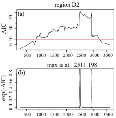
2752.9 3898.0 3.0 0.063 0.92 0.1086 0.60 1.01 10.2 9.4(548) 100.0 3882.0 3.0 0.070 544.76 0.1382 1.86 1.19 1105.6
D2 100.0 2511.2 3.0 0.047 0.2715 0.0601 0.34 0.89 1042.4
2511.2 3882.0 3.0 0.058 1480.3 0.1542 2.39 1.11 63.2 9.7(920) 100.0 4901.0 2.2 0.025 750.43 0.0004 1.84 0.99 1635.2
E 100.0 2780.0 2.2 0.020 455.52 0.0001 1.70 0.96 1633.4
2780.0 4901.0 2.2 0.040 858.73 0.0026 2.01 1.21 1.8 9.4(545) F 0.1 1983.0 2.5 0.019 803.37 0.0004 2.86 0.91 -1076.3 (1260) G 0.1 1922.0 2.0 0.012 7.22 0.0194 2.27 1.10 -2761.4 (784) 200.0 4490.0 1.5 0.013 40.87 0.0018 2.01 1.32 445.0
H1 200.0 2690.9 1.5 0.016 17.91 0.0008 1.73 1.26 435.6
2500.0 4490.0 1.5 0.010 -- -- -- -- 9.8 7.9(108) 1.0 4490.0 1.5 0.000 23.52 0.0287 1.66 1.25 -4830.0
19
H2 1.0 1247.6 1.5 0.000 25.21 0.0333 1.68 1.24 -4857.0
1247.6 4490.0 1.5 0.010 -- -- -- -- 26.9
9.8 (1048) 150.0 4404.0 1.5 0.010 1.141 0.0015 0.87 1.15 521.5
H3 150.0 4086.0 1.5 0.009 0.0133 0.0013 0.00 1.11 492.5
4086.0 4404.0 1.5 0.049 2.287 0.0021 1.00 1.22 29.0 8.3(192) Table 2-3. The MLE and AIC values of the ETAS model.
The data of the region A ~ D are taken for the period from October 1997 till 13 June 2008. The period for the region E is from 1995, the region E from 26 May 2003, the region G from 26 July 2003, and the region H from October 1996, all till 13 June 2008. The S and T represent the periods through which the ETAS model is fitted to each region, counted in days from the beginning of the data period. Mz indicates the cut-off magnitude. For each region except for F and G, the first row lists the result of ETAS model fitted to the entire period, the second row till the change-point, and the third from the change-point. In the AIC column, the first row in each region is AIC0, the second is AIC1+ AIC2: the AIC sum of two models separated by a change-point. The third row shows ΔAIC = AIC0 – (AIC1+ AIC2). The last column shows twice the degree of freedom in searching a change-point (see text and Appendix A). Here, ΔAIC > 2q indicates that the searched change point is significant.
The Japan Sea region (region A in Fig. 2-3 and 2-4a) is largely in the stress shadow (i.e., the region where ∆CFS is negative). The large cluster of earthquakes dominating the central part of this region consists of aftershocks of the 1983 Central Japan Sea
earthquake of M7.7. Therefore, we regard the mainshock fault model [Kanamori and Astiz, 1985; see Table 2-2] as the representative receiver fault of this region. The
~150-km NS trending seismic cluster contains large earthquakes of M5.4 and M5.3 that successively occurred on 18 October 2005 associated with a very short-term cluster, after which however the seismicity rate lowered, or became quiet, relative to the predicted rate (Fig. 2-4b and c). This is clearly seen by the lowered slope of the cumulative curve. This seismicity change is significant in terms of AIC as described in Table 2-3. In Fig. 2-5 (a), the solid curve shows the improved amount of AIC by setting a change-point at each interval of events, without taking into account the penalty of searching a change-point (i.e., AIC1+ AIC2- AIC0 by the notation of chapter 2-2). The red horizontal line represents the penalty of searching a change-point from the data
21
alone. We hence can say any point as a significant change-point as long as the solid curve there is above the red line. Our choices here and the following regions are the ones with the best AICs. Here the change-point with the best AIC is at T=2936.594. The curve in Fig. 2-5 (b) is the scaled AIC, in such a way as
exp
AIC
1 AIC2 AIC0
2
,so that it shapes like standard normal around its peak. The error bars in Fig. 2-4 (b) is calculated from this scaled AIC, by regarding it as a probability density.
Figure 2-4, a~c. The focal polygonal region in (a) corresponds to A region in Fig. 2. The red and blue contours indicate positive and negative CFS increments (cf., Table 2), respectively, with logarithmically equidistant values due to the assumed slip on the fault as the source (see Table 1 and Fig. 2). The right panels show the empirical (black) and theoretical (red) cumulative curves with respect to regular (b) and transformed (c) time for the occurrence sequence of earthquakes. The theoretical curves (red) are fitted for the period till the change-point (the middle vertical dashed line; see Table 1) then extrapolated to cover the entire period. The colored bars on the panel (b) represent change-point’s confidence intervals of 68.3% (red), 95.5% (green) and 99.7% (blue), which are (2804, 2937), (2738, 2937), and (2735, 2937),
21
respectively.
Figure 2-5. (a) The solid curve is the difference of the AIC; ΔAIC= AIC0-(AIC1+ AIC2), and the red horizontal line is 2q. The unit in horizontal axis is a day. (b) The solid curve is exp(-ΔAIC/2). The dashed lines are error boundaries in Fig. 2-4 (b).
The inland area of Aomori and Iwate prefecture (B region in Fig. 2-3, and 2-6 (a)) to the north of the source has positive ∆CFS values throughout the entire region, where we assumed the north-south striking reverse faults for the receivers in the northern Tohoku inland. We fitted the earthquake sequence after September 1998, or T = 330 days from the beginning, till the end to avoid the beginning period of volcanic swarm [Nishimura et al., 2001; Ueki and Miura, 2002; Nishimura et al., 2005] which has very different ETAS parameter values from those of the tectonic seismic activity. In this case, the seismic sequence activated relative to the predicted ETAS rate since the middle of 2003 (see Fig. 2-6 (b) and (c)), which is very significant according to the AIC difference.
23
As can be seen in Fig. 2-7, a significant change-point ranges wide, with the best being at T=2203.631.
Figure 2-6, a~c. The seismicity in B region, where captions are the same as Fig. 2-2. The colored confidence intervals of 68.3%, 95.5% and 99.7% are (2153, 2259), (1681, 2363) and (1540, 2599), respectively.
23
Figure 2-7. (a) The solid curve is ΔAIC= AIC0-(AIC1+ AIC2), and the red horizontal line is 2q. (b) The scaled AIC.
In the Pacific upper plate boundary zones (regions C1 and C2 in Fig. 2-3 and 2-8 (a)) and the outer rise zones (regions D1 and D2 in Fig. 2-3 and 2-8 (a)), the seismicity appears to change consistently with the ∆CFS sign, where we assumed typical reverse faulting of the plate boundary and normal faulting in outer rise area, respectively. The activation in the region C1 of Fig. 2-3 is not significant whether or not we take account of the change-point penalty 2q over whole period (see Fig. 2-9), while the lowering in the region C2 on the other hand is significant in a narrow interval around T=2658.546 (see Fig. 2-10); the observed swarm of around August 2005 (T = 2800 days) in C2 region does not catch up with what the earlier seismicity predicts. Similar patterns can be observed in the outer rise regions of D1 and D2. D1 has a significant change-point within narrow range around T=2752.202, whereas D2 has wide range of significance (Fig. 2-12 and 13). In the region D2 especially the prediction by the earlier seismicity fails to follow the observed swarms at around T = 2900 days. Because of the regions
25
being offshore, we have to set higher cut-off magnitude, Mz, for these regions than those in inland regions.
Figure 2-8, a~c. The seismicity in C1 (panel (b1) and (c1)) and C2 (panel (b2) and (c2)) region. The colored confidence intervals of 68.3%, 95.5% and 99.7% for the region C1 are (2209, 2474), (2190, 3327) and (942, 3327), respectively. For the region C2, they are (2006, 2858), (1956, 2867) and (1802, 3019), respectively.
25
Figure 2-9. The solid curve is ΔAIC= AIC0-(AIC1+ AIC2).
27 Figure 2-10. The solid curve is ΔAIC= AIC0-(AIC1+ AIC2), and the red horizontal line is 2q.
27
Figure 2-11, a~c. (a) The seismicity in D1(pane l(b1) and (c1)) and D2 (panel (b2) and (c2)) region. The colored confidence intervals of 68.3%, 95.5% and 99.7% for the region D1 are (2739, 2753), (2621, 3025) and (2326, 3132). For the region D2, they are (2511, 2498), (2484, 2511) and (2483, 2936), respectively.
29 Figure 2-12. The solid curve is ΔAIC= AIC0-(AIC1+ AIC2), and the red horizontal line is 2q.
29
Figure 2-13. The solid curve is ΔAIC= AIC0-(AIC1+ AIC2), and the red horizontal line is 2q.
The southwest neighboring region of the fault (E region in Fig. 2-3 and 2-14 (a)) is also the area where the seismicity is affected by pre-, co- and postseismic slips due to the nearby 2004 Chuetsu Earthquake of Mw6.6 [Ogata, 2005]. This region is totally neutral relative to the Chuetsu earthquake source including regions of both positive and
negative ∆CFS, but it is entirely positive in ∆CFS relative to the Iwate-Miyagi Nairiku slip. Here we assumed NE-trending reverse faulting as the receiver fault corresponding to the general trend of active faults in this area. However, the ETAS analysis of its change-point effect is not significant in AIC whether or not the change-point penalty of 2q is taken into consideration (see Fig. 2-15). We will revisit this problem later, in Ch 2-9.
31 Figure 2-14, a~c. The seismicity in E region. The colored confidence intervals of 68.3%, 95.5% and 99.7% are (2658, 3193), (2658, 3976) and (2101, 4073), respectively.
31
Figure 2-15. The solid curve is ΔAIC= AIC0-(AIC1+ AIC2), and the red horizontal line is 2q.
The small regions of F and G of Fig. 2-3 covers major aftershock clusters of the 2003 southern Sanriku coast earthquake of M7.0 (Fig. 2-16 (a)) and northern Miyagi-Ken earthquake of M6.4 (Fig. 2-17 (a)), respectively. For these regions we focus on their aftershock activity. There is no significant change-point since each cluster spreads across or near the boundary of changing sign in ∆CFS: see Table 2-2 and GSI [2004] for respective fault angles of the main shock.
33 Figure 2-16. The seismicity in F region.
33
Figure 2-17. The seismicity in G region.
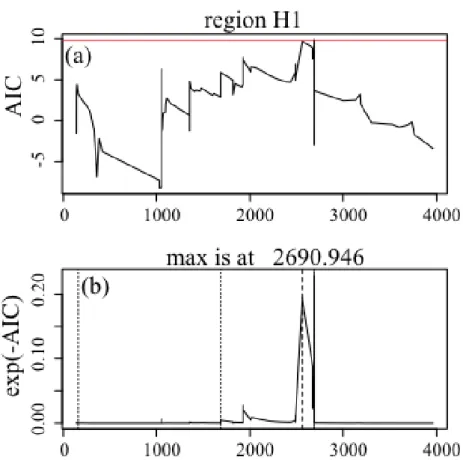
The clusters in the near field to the source can be divided up into three small regions (regions H1, H2, H3 in Fig. 2-3, and 18(a), 20(a), 22(a), respectively), each of which has a unique seismicity change. For the receiver fault angles of each region, we have used a fault mechanism of the largest earthquake available from F-net catalog [see the inset map of Fig. 2-2 and Table 2-2; NIED, 2010], and ∆CFS pattern does not change much with the alternative conjugate mechanism. Possible high fluid pressure associated with hydrothermal activity in the volcanic regions may have reduced the apparent friction coefficient, but the ∆CFS patterns with such low friction still remain similar to those with μ’=0.4 which is assumed throughout the present paper. The clusters in the regions H1 and H2 of Fig. 2-2 fall in stress shadow, and accordingly show quiescence as seen in Fig. 2-18 and 2-20, which are significant in terms of the AIC. The former region has narrow range of significance around T=2690.946, whereas it ranges widely in the latter (Fig. 2-19 and 21). From the extrapolated ETAS cumulative curve after the change-point in Fig. 2-20, the quiescence relative to the theoretical cumulative curve is
35
hard to see unless the figure is magnified substantially. However, the region has had only a few earthquakes for a long period over 2000 days after 2001, which makes the quiescence very significant in the sense of the AIC difference.
Figure 2-18, a~c. The seismicity for H1 region. The colored confidence intervals of 68.3%, 95.5% and 99.7% are (2563, 2691), (1687, 2691) and (160, 2691), respectively.
35
Figure 2-19. The solid curve is ΔAIC= AIC0-(AIC1+ AIC2), and the red horizontal line is 2q.
37 Figure 2-20, a~c. The seismicity in H2 region. The colored confidence intervals of 68.3%, 95.5% and 99.7% are (1053, 1227) and (342, 1227) and (299, 1248), respectively.
37
Figure 2-21. The solid curve is ΔAIC= AIC0-(AIC1+ AIC2), and the red horizontal line is 2q.
39 Figure 2-22, a~c. The seismicity in H3 region. The colored confidence intervals of 68.3%, 95.5% and 99.7% are (4087, 4129), (4022, 4168) and (3920, 4198), respectively.
39
Figure 2-23. The solid curve is ΔAIC= AIC0-(AIC1+ AIC2), and the red horizontal line is 2q.
Region H3 has been activated since around 2007 (see Fig.2-22 (b) and (c)) while this region is entirely in stress shadow under the assumed slip (Fig.2-24 (a)). In the figure 2-22(a), we assumed slips in the deeper extension of the southern fragment. We will verify this assumption of slips in deeper extension in the next section, with the observed crustal deformation by GPS network. If we focus on the period before this activation, we see clear quiescence after 150 days from the beginning of 1996. Fig.2-24 (b1) and (c1) show ETAS estimate in [S,T]=[1,150], while (b2) and (c2) show estimate in [S,T]=[82.72, 150]. Both change point at T=150 improves the AIC by 31 and 24.4 respectively. Note that the earlier half of this estimation period, before T=82.72, includes swarm like events, hence including that period or not changes largely the estimated parameters. One observation deserves mentioning; only a few aftershocks followed the M4.4 at around 2006. This is clearly be seen by the extrapolated ETAS fittings and clearly suggests quiescence. Since this region is very close to the source, slight slip may have enough effect on seismicity changes here, while leaving other relatively far regions unaffected. We end this section by adding that this assumption, of
41
active site having moved deeper along the fault, does not conflict the detected changes in seismicity in the other two nearby regions H1 and H2. Fig.2-25 shows the ∆CFS ‘s in both regions still being in shadow, or neutral.
Figure 2-24, (a) ∆CFS is cast by the slips in the southern fragment. (b1,c1) ETAS estimation (red) from from T=1 till T=150, which parameters are (0.0267, 0.0554, 0.0202, 0.936, 1.252). (b2,c2) ETAS estimation (red) from from T=82.72, (after relatively large M3.9) till T=150, which parameters are (0.0, 0.00498, 0.0067, 2.588, 0.957).
41
Figure 2-25. ∆CFS for H1(left) and H2(right), with the source that of deeper extension of the southern fault.
In summary, the solid blue and red zone boundaries in Fig. 2-3 show significant relative quiescence and activation, while solid greens show activities just as predicted by the single ETAS model. Dashed boundaries show that the anomaly is not significant by the AIC. These results indicate that the seismicity in most zones had changed consistently with the ∆CFS calculated from the pre-existing stress field in this region, from several years before the M7.0 occurred.
2-5-4. Crustal deformations by GPS network
The data from the GPS Earth Observation Network System (GEONET) by the Geographical Survey Institute of Japan [GSI, 2009a] are used to observe the surface deformations. The GEONET stations are located at roughly every 20km, providing their daily coordinates since 1996 for the earliest stations. The data are also sensitive to any non-crustal disturbances such as maintenance on and around the stations, as well as shading by surrounding trees, hence we removed any such disturbances of known causes if found.
In this study, we consider baseline distances between the stations because we expect that the baseline distance, in comparison with the displacement of the station locations relative to a station set as the coordinates origin, can cancel or reduce the various
43
common effects of wide tectonic crustal movement, so that we can concentrate on the analysis of relative displacements around the source fault.
During a number of years before the focal earthquake, several stations around the considered fault were installed for the purpose of monitoring magma source in volcanic activity. In particular, the station "Kurikoma2" (station H in Table 2-4 and in the inset of Fig. 2-26) is located at the foothills of the Kurikoma volcanic mountain, which turned out to be also right atop the focal fault. During about the same period of our concern with the seismic anomaly, some anomalous displacement of the Kurikoma2 station was observed by the GSI, who suspected volcanic activation beneath the Kurikoma2 station behind this displacement, installed an additional temporary station nearby to confirm the geodetic anomaly [GSI, 2008, Internal report for the Coordinating Committee for Prediction of Volcanic Eruptions at 8 October 2008; also see JMA, 2008].
The data from Kurikoma2 station became available from July 2004, and Fig. 2-26 shows that Kurikoma2 station moved toward southeast relative to its neighboring stations over the earlier 3 years during the period from July 2004 to November 2007. In the inset figure, arrows and numbers represent the average changed distances per year, calculated by using the difference of distances over the periods in Table 2-4 [Kumazawa et al., 2009c and d]. Meanwhile, GSI [2009b] reported that these particular movements observed at Kurikoma2 were due to neither instrumental error nor very local event such as land slide, by means of the additional observation of the temporary station (green dot in the inset of Fig. 2-26) on another ridge 500 meters east of Kurikoma2. The
background for the Kurikoma2 and temporary stations installation was to monitor subterranean volcanic activities around the Kurikoma volcanic mountain. However, no sign of volcanic activity was found even after the June 2008 mainshock [JMA, 2008] up to the present. Also, GSI [2010] reported, by an independent analysis, that the model [Kumazawa et al., 2009a, 2009b] with slip rate of 2 cm/year could explain the transient crustal deformation around this region without the possible volcanic magma migration. Thus, these observations are strong collateral evidence that precursory slips took place in the southern segment.
43
Station Name ID lon(deg.) lat(deg.) Baseline change (mm)
A Isawa 970796 140.9885 39.1270 1.8
B Higashinaruse 20928 140.7150 39.1462 0.8
C Minase 950193 140.6296 39.0519 6.7
D Ogachi 20929 140.4473 39.0544 5.0
E Mogami 20931 140.4973 38.7522 -0.8
F Naruko 950174 140.8016 38.7489 -3.5
G Kurikoma 950173 140.9906 38.8153 -9.8 H Kurikoma2 20913 140.8332 38.9340
I Yuzawa 960554 140.5067 39.1991
Figure 2-4. The focal polygonal region in (a) corresponds to A region in Fig. 2-2. The red and blue contours indicate positive and negative CFS increments (cf., Table 2-2), respectively, with logarithmically equidistant values due to the assumed slip on the fault as the source (see Table 2-1 and Fig. 2-2). The right panels show the empirical (black) and theoretical (red) cumulative curves with respect to regular (b) and transformed (c) time for the occurrence sequence of earthquakes. The theoretical curves (red) are fitted for the period till the change-point (the middle vertical dashed line; see Table 1) then extrapolated to cover the entire period. The colored bars on the panel (b) represent change-point’s confidence intervals of 68.3% (red), 95.5% (green) and 99.7% (blue), which are (2804, 2937), (2738, 2937), and (2735, 2937), respectively.
45 Figure 2-26. Daily time series (grey and blue dots) of the baseline distance changes from Kurikoma2 to each stations in the inset, over 4 years’ period from July 2004 till 13 June 2008 (just before the rupture). The details of the stations are listed in Table 2-4. The thick curves link medians of moving window over a month (31 days) of base-line distance changes, and thin straight lines illustrate their linear trends. The vertical red lines correspond to the timing of the 16 Aug 2005 Miyagi-Ken Oki earthquake of M7.1 and
45
the 14 Jun 2008 Iwate-Miyagi Inland earthquake of M7.2. In the inset map, the numbers between station H (Kurikoma2) and each other station show changed distance in milli-meters per-year during the period with overlaid liner trends, which details are listed in Table 2-4. The right end arrows show the directions of jumps at time of the 2008 mainshock.
Furthermore, Fig. 2-26 also indicates the distance changes within the last two years preceding the mainshock. Notably, the slopes of the linear trends of the baseline distances have changed after around the end of 2006. This is also true for the baseline between Krikoma and Krikoma2, even taking account of the distinct postseismic deformation due to the M7.2 Miyagi-Ken-Oki earthquake of 16 Aug 2005 (the vertical red line in Fig. 2-26). These changes in trends suggest that the movement of
Kurikoma2 relative to the surrounding stations either became relatively silent or moved toward northwest which counters their earlier trends. It appears that Kurikoma2 and the southeastern two stations become more stationary, while the northwestern two stations are weakly enhanced to move toward Kurikoma2. Thus the Kurikoma2 station seems to move relatively toward northwest.
2-6. Discussion for change-point analysis
We are concerned with the sign of the CFS increment of the region although the ranges of the CFS increments are very wide depending on the area size of the region as given in Table 2-2. This paper does not evaluate the quantitative effect of ΔCFS but assumes that there is no threshold value of ΔCFS capable of affecting seismic changes. The stress changes due to aseismic slip can be small values on the order of millibars (10-4 MPa) or less, which are comparable to or even smaller than fluctuations in daily earth tides. However, unlike the tidal changes that are oscillatory and too brief to nucleate abundant earthquakes [Dieterich, 1988; Beeler and Lockner, 2003], this kind of slips is, possibly intermittently, one way. Hence the number of actual and potential earthquakes of small sizes to be triggered or inhibited in a seismic zone can be substantially many to statistically detect significant activation and quiescence relative to the ETAS model in the respective zones under such small Coulomb stress changes.