Sequential Internet Auctions with Different Ending Rules
Toshihiro Tsuchihashi∗†
March 2011
Abstract
Two ending rules, a soft close and a hard close, exist in Internet auctions. The hard close auction involves a fixed deadline, while the deadline in the soft close auction may be extended if at least one bid is submitted in the final few minutes. Thus, the soft close allows buyers to submit ofter observing the opponent’s bids even in the last minutes. Ending rules change both the seller’s and the buyers’ strategies. In a sequential auction with the soft close, buyers have a stronger incentive to wait for low reserve prices in the future, and a seller chooses lower reserve prices.
1 Introduction
Since Onsale and eBay started Internet auctions in 1995, the number of items and the total value of transactions have been growing at a high rate. Internet auctions provide sellers many inherent options that traditional auction houses such as Sotheby’s and Christie’s do not have. Lucking-Reiley (2000) discusses the options in his detailed survey of Internet auctions. Yahoo! Japan auction allows sellers to choose one of two rules for ending auctions, a soft close and a hard close in each auction.1 A hard close auction finishes at a predetermined time, while a soft close auction may not. In the soft close auction, the deadline is extended a few minutes if at least one bid is submitted in the final few minutes (ten minutes in Yahoo! Japan’s auctions), and the auction finishes if the final minutes pass without any bids.2 The important feature
∗Department of Economics, Daito Bunka University; 560, Iwadono, Higashi Matsuyama, Saitama, Japan 355-8501; E-mail:[email protected]
†I am very grateful to Yossi Spiegel, Rudolf Muller, Ron Lavi, Olivier Compte and attendees at the Hitotsub- ashi G-COE Conference on Mechanism Design, Hitotsubashi Game Theory Workshop and 14th DC conference for helpful comments and suggestions. I am truly indebted to my supervisor Akira Okada for his invaluable guidance. Any remaining errors are of course my own responsibility.
1While Yahoo! Japan auctions allow the sellers to choose an ending rule, the sellers cannot choose the rule in eBay auctions and Amazon auctions, well-known Internet auctions. Yahoo! in the US also allowed the sellers to choose the ending rule, but Yahoo! ended their auction services in September 2007.
2eBay adopts a hard close while Amazon adopts a soft close.
of the soft close auction is that the buyers always have opportunities to submit bids after observing the other buyers’ bids because of the extended deadline. In the hard close auction, on the other hand, a buyer loses the opportunity to submit a bid if he takes a wait-and-see attitude but the other buyers submit a bid at the last moment. This situation may arise in actual Internet auctions because the auction may be repeatedly held and the buyers can often expect that the reserve prices will go down in the future.
This paper provides a model of the Internet soft close auction as an infinitely sequential auction, where each period is a modified sealed-bid-second-price auction and the seller posts a reserve price at the beginning of each period under the independent private value (IPV) assumption. Using the model, we discuss which rule brings the highest revenue to the seller, and how the seller theoretically chooses the optimal reserve price in each auction. Finally, we see starting price data similar to reserve prices gathered from Yahoo! Japan auctions.
We obtain two results. First, the seller posts a higher reserve price in hard close auctions than in soft close auctions. The buyers in soft close auctions have opportunities to submit bids after observing the other buyers’ bids. Thus, the buyers have stronger incentives to wait for lower reserve prices in the future in soft close auctions than in hard close auctions. Knowing the buyers’ attitudes, the seller posts a lower reserve price in soft close auctions than in hard close auctions, preventing the expected revenue from being discounted. The data show the difference among reserve prices in different auctions, which is consistent with the second result above, although the difference is not statistically significant.
Second, revenue equivalence holds between hard close auctions and soft close auctions. Because the seller chooses different reserve prices depending on the buyers’ incentives to wait for lower reserve prices in the different auctions, the timing of the item to be sold is independent of ending rules, leading to revenue equivalence.
Roth and Ockenfels (2002) and Ockenfels and Roth (2006) also analyze the two ending rules. Ockenfels and Roth (2006) consider a modified English auction where auctions are held during the period [0, 1], but any bids may fail to transmit at t = 1. The auctions ends after t = 1 in the hard close auctions, while the extra duration [1, 2] appears if at least one bid is successfully transmitted at t = 1 in the soft close auctions. Roth and Ockenfels (2002) and Ockenfels and Roth (2006) show that late bidding or “sniping”, a certain buyer’s bidding
strategy, can construct the equilibrium in the hard close auctions but cannot in the soft close auctions. The theoretical result is consistent with observations in eBay auctions and Amazon auctions.3
However, they do not consider the following two important points. First, they do not explicitly analyze the seller’s strategy. In Internet auctions, the seller usually chooses a starting price/reserve price in each auction. Because the ending rule can change the structure of games, the seller can choose different prices depending on the ending rules, leading to different best responses of the buyers.4
Second, a model of sequential auctions better represents Internet auctions than a one-shot model. The seller can hold the auction whenever she wants to sell her item, and she can quickly re-auction the item with few costs even when the item remains unsold. In this sense, this feature of Internet auctions is well captured by the model of sequential auctions with a single item, which is introduced by McAfee and Vincent (1997).5 In this paper, we construct a model of Internet soft close auctions by developing McAfee and Vincent’s (1997) sequential auctions model and compare reserve prices. McAfee and Vincent (1997) analyze sequential auctions with a single item in which the stage game is a sealed-bid-second-price and a sealed- bid-first-price auction under the IPV assumption. In their model, a seller posts a reserve price at the beginning of each period. In equilibrium, the seller posts a high reserve price in the first period and decreases the reserve price in subsequent periods.6 Each buyer faces a trade-off between submitting a bid in the current period and waiting for lower prices in the future.
In another study, Grant et al. (2006) discuss repeated auctions in the IPV context in which
3Ariely et al. (2006) construct laboratory experiments of hard close auctions and soft close auctions, and they show that more late bidding occurs in hard close auctions than in soft close auctions.
4A reserve price is widely studied theoretically and empirically. Myerson (1981) and Riley and Samuelson (1981) are the first to consider an optimal auction, where a reserve price strictly increases a seller’s revenue. Reserve prices are often kept secret. In this case, a relation between reserve prices and a seller’s commitment be- comes an important issue. Vincent (1995) studies a secret reserve price, and Carey (1993) analyzes a false reserve price. Bajari and Hortacsu (2003) empirically consider a reserve price, by using data from eBay. They report that sufficiently lower reserve prices (minimum bids) bring a seller higher revenues. Hoppe (2008) constructs an experiment of multiple auctions, and he also obtains the similar result.
5There are also many studies of sequential auctions in which a seller has many identical items and sequentially sells one unit of the item in each auction. Each buyer has single-unit demand and exits from the auction after getting the item. The winning prices theoretically drift upward (Weber (1983), Milgrom and Weber (2000)), but they have a tendency to drift downward in real auctions (Ashenfelter (1989)).
6In a bargaining game under one-sided or two-sided uncertainty, similar results are obtained. The offer prices are consequently decreasing. See Samuelson (1984), Fudenberg et al. (1985) and Gul et al. (1986).
a seller chooses both the reserve price and a duration for each auction. In their model, a seller cannot change the reserve price once she chooses it. They adopt an English auction as a stage game in which bidders appear according to a random (Poisson) arrival process.
This paper is organized as follows. Section 2 presents the model. Section 3 considers the one shot case and Section 4 considers the sequential case. Section 5 analyzes stationary linear equilibria. Section 6 shows main results, and Section 7 concludes. All proofs are provided in the Appendix.
2 The Model
A seller wants to sell a single item to n potential buyers, indexed by i, via a sequential second- price auction with a soft close ending rule. The seller evaluates zero to the item. Buyer i’s value for the item vi is his private information, and identically and independently drawn from [0, 1] according to the distribution function F (·), with positive density f (·). Let G(·) denote the distribution function of the highest order statistics v(1)−i = max{v1, · · · , vi−1, vi+1, · · · , vn} for a given i; that is, G(v) = [F (v)]n−1. Denote the density function by g(·).
The sequential auction consists of infinite periods, indexed by t, and each period consists of two potential stages. In period t, at the beginning of the first stage, the seller chooses a reserve price rt. Buyers then simultaneously submit bids. We call the bid above the reserve price a serious bid, as in McAfee and Vincent (1997). We assume that all bids are observable to the buyers and the seller, but only serious bids can be accepted by the seller. Any bid below the reserve price are not accepted by the seller; thus, such bid reflects the buyer’s wait-and-see attitude.
If no serious bid is submitted in the first stage, then the auction moves on to the next period t + 1. However, if at least one buyer submits a serious bid, then the second stage starts. In the second stage, the seller cannot post a new reserve price. This means that at the beginning of the first stage the seller can commit not to reserve price in the second stage. We adopt this setting because in an actual Internet auction (Yahoo!) a seller cannot post a new reserve price in any extended duration. In the second stage, the buyers simultaneously submit bids again given the current price, which is the higher of the second highest bid and the reserve price. After the second stage, the auction ends. The buyer with the highest serious bid throughout
the first and the second stages gets the item, and pays a price p, which is the higher of the second highest bid and the reserve price.
The two-stage setting captures the feature of extension of soft close auctions where all buyers surely get a chance to submit a serious bid after they know the auction ends in the current period because of the opponent’s serious bid. Hard close auctions, however, may not give the chance to the buyers due to sniping.
The second stage starts if and only if the auction ends with certainty in the current period. Thus, only the final period faces the second stage, while the other periods consist of only the first stages.7 8
Both the seller’s and the buyers’ payoffs are discounted by a common discounting factor δ ∈ (0, 1). That is, the seller’s payoff is δt−1p and the buyer i’s payoff is δt−1(vi− p) if the auction ends at period t and the payment is p.
We study a perfect Bayesian equilibrium (PBE) with the following property. In the first stage, buyers follow a stationary symmetric bidding strategy given by a pair of functions (b, β).
• A bid is determined by the function b(·) which is a strictly increasing function, if a reserve price is below some threshold v∗i ∈ [0, 1]; otherwise, buyer i submits zero.
• The threshold vi∗ is determined by the function β(·) which is strictly increasing in the buyer’s value.
That is, in the first stage, if a reserve price rtsatisfies rt≤ v∗i = β(vi), then the buyer i submits a serious bid b(vi), while if rt> v∗i, then b(vi) = 0. In the second stage, buyers follow a weakly dominant strategy in which they truthfully submit their values.
A seller follows a stationary strategy given by a strictly increasing function α(·) to determine a reserve price rt. Suppose ¯v ∈ (0, 1). If the seller believes that the values lie between [0, ¯v) with a distribution function F (·)/F (¯v) at the beginning of period t, then she chooses a reserve price rt such that any buyer with value at or above α(¯v) would submit a serious bid. We
7Ockenfels and Roth (2006) consider a one-shot English auction with two stages. In their model, an auction is held during the period [0, 1]. The first stage is [0, 1], where any buyer can reply to other bids. The second stage is {1}, where any buyer cannot reply to other bids.
8Use of only two stages does not affect the generality of our results. The key is that the second stage is the same as a standard sealed-bid-second-price auction because the auction surely ends in the current period. Thus, even if we add a third stage, the additional third stage cannot affect the outcome.
refer to α(¯v) = v∗t as a cutoff value induced by the reserve price rt. We assume the seller’s following belief. On the equilibrium path, if no buyer submits a serious bid against a reserve price rt with a cutoff value vt∗, i.e. rt = β(vt∗) in period t, then the seller updates her belief by Bayes rule; thus, she believes that all values lie between [0, vt∗) according to a distribution function F (·)/F (vt∗) in period t + 1. The seller believes that all values lie between [0, 1], off the equilibrium path.
3 One-period case
In this section, we consider both a hard close auction with only one period and a soft close auction with only one period. A hard close auction with only one period is identical to a standard sealed-bid-second-price auction. Given a reserve price r, it is a weakly dominant strategy for buyer i to submit a serious bid vi truthfully. Conditional on winning, the buyer i’s payment is equal to the reserve price r if his opponents do not submit any serious bids, while his payment is the second highest value if some opponents submit serious bids. Therefore, the expected payment of the buyer i with vi≥ r is given by:
rG(r) +
∫ vi
r
ydG(y),
where y = v(1)−i, the highest order statistic for buyer i. The first term is the expected payment in the case that the second highest buyer’s value y is below r, and the second term is the expected payment in the case of y > r. The ex ante expected payment of each buyer is given
by: ∫ 1
r
[rG(r) +
∫ x r
ydG(y)]dF (x) = r(1 − F (r))G(r) +
∫ 1 r
v(1 − F (v))dG(v). By choosing a reserve price r, the seller obtains the following expected payoff:
Π0(r) = n[r(1 − F (r))G(r) +
∫ 1
r
v(1 − F (v))dG(v)]. Define:
J(v) = v −1 − F (v)
f (v) . (1)
We assume that J(v) is increasing in v (regularity assumption). In this setting, the optimal reserve price r0 which maximizes Π0(r) is given by:
r0=
{J−1(0) if J(0) < 0
0 otherwise. (2)
If the values are uniformly distributed on [0, 1], i.e. F (vi) = vi, then the optimal reserve price r0 is set as r0 = 1/2 since the following holds:
r0= J−1(0) ⇔ r0 = 1 − F (r0) f (r0) .
A soft close auction with only one period is a modified sealed-bid-second-price auction, which has potentially two stages. If no buyer submits a bid against a reserve price r in the first stage, then the auction ends, and all seller and buyers obtain zero payoff. Therefore, buyer i should submit a serious bid b ≤ vi in the first stage independent of the opponents’ behavior if a reserve price is at or below vi, i.e. r ≤ vi, since the bid brings the buyer i a chance to submit a serious bid in the second stage, leading to a non-negative payoff. Note that any serious bid b > vi cannot be optimal for the buyer i, since he cannot submit any bids below b in the second stage. In this case, the payment may be above his value vi even if he wins the auction. As can be seen below, truthful bid in the first stage is not a weakly dominant strategy in sequential auctions.
The second stage is identical to a standard sealed-bid-second-price auction. Thus, in the second stage, it is a weakly dominant strategy for buyer i to submit a serious bid vi truthfully. After all, the seller faces the same optimization problem as that of a standard sealed-bid- second-price auction; thus, the optimal reserve price is given by r0.9
Therefore, if the auctions consists of only one period, then the ending rules do not influence the optimal reserve price.
9The result relies on the assumption that the seller can commit not to a new reserve price in the second stage. Caillaud and Mezzetti (2004) consider a two-stages ascending auction where the seller chooses a reserve price at the beginning of each stage. That is, at the beginning of the first stage, the seller cannot commit to the second stage’s reserve price r2. They show that, due to the lack of commitment, the seller optimally chooses a reserve price r1̸= r0 such that less buyers submit serious bids in the first stage than in the optimal auction, while she chooses a reserve price r2< r0 such that more buyers submit serious bids in the second stage than in the optimal auction. Furthermore, the seller’s payoff in the two-stages ascending auction is strictly lower than in the optimal two-periods auction under full commitment.
4 Sequential soft close auction
In this section, by developing McAfee and Vincent’s (1997) model, we consider a sequential soft close auction that has potentially infinite periods. As the one-period case above, in any period t, buyer i should optimally submit his true value vi as a serious bid in the second stage. Therefore, we have to consider the buyer’s optimal behavior in the first stage. We define a truthful cutoff strategy in the following way.
Definition 1 (Truthful cutoff strategy). Buyer i’s strategy (b, β) is a truthful cutoff strat- egy if a strictly increasing function β(vi) determines a threshold vi∗, and he truthfully submits a serious bid if a reserve price rt is at or below the threshold in period t, that is:
b(vi) =
{vi if rt≤ β(vi) = vi∗ 0 otherwise.
We prove first that in any symmetric PBE, given a threshold vi∗, buyer i optimally submits a serious bid which is equal to or lower than his true value vi against a reserve price rt≤ vi∗.
Lemma 1. Suppose that a strictly increasing function β(·) determines a threshold v∗i for buyer i in equilibrium. In any PBE, if a reserve price rtis equal to or lower than the threshold in period t, then buyer i optimally submits a serious bid which is equal to or lower than his true value in the first stage. That is, b(vi) ≤ vi for all i such that rt≤ v∗i.
The truthful bid b(vi) = viinduces any equilibrium outcome where all buyers submit serious bids below their true value b(vi) < vi in the first stage, because all buyers truthfully submit in the second stage. Therefore, we restrict our attention to an equilibrium in which all buyers with values at or above the cutoff value submit according to the truthful cutoff strategy in the first stage. The threshold is determined as follows.
Buyer Now, we consider the buyer’s expected payoff. In period t, given a reserve price rt
with the corresponding cutoff value vt∗, any buyer with value above v∗t submits his true value in the first stage, leading to the second stage. All buyers truthfully submit in the second stage.
Therefore, buyer i wins the auction if and only if he has the highest value among all buyers (with probability G(vi)), and his payment is equal to reserve price rt if the second highest bid does not reach rt, while his payment is the second highest value of the remaining buyers otherwise, as in the standard sealed-bid-second-price auction. Conditional on winning, buyer i obtains the expected payoff given by:
viG(vi) −[rtG(rt) +
∫ vi
rt
ydG(y)].
If no buyer submits a serious bid in period t, then the auction moves on to period t + 1, where the seller posts a reserve price rt+1at the beginning of the first stage. Buyer i submits a serious bid in period t + 1 in the event of no sale in period t, his expected payoff is given by:
δ(viG(vi) −[rt+1G(rt+1) +
∫ vi
rt+1
ydG(y)]).
Because the buyer with value equal to the cutoff value vt∗ should be indifferent between sub- mitting in period t and submitting in period t + 1 in equilibrium, we obtain the following equation:
vt∗G(vt∗) −[rtG(rt) +
∫ v∗t
rt
ydG(y)]= δ(vt∗G(vt∗) −[rt+1G(rt+1) +
∫ v∗t
rt+1
ydG(y)]). (3) According to the truthful cutoff strategy, buyers with value v > vt∗ submit in the current period t, while buyers with value v < vt∗ do not. As shown in Lemma 2, the truthful cutoff strategy constructs a PBE. However, note that the truthful cutoff strategy is not a weakly dominant strategy.
Lemma 2. Given the cutoff value defined by (3), the truthful cutoff strategy constructs a PBE.
Seller Next, we consider the seller’s behavior. The seller chooses a sequence of reserve prices {rt}t=1,2,···. However, given the buyer’s truthful cutoff strategy, we can consider a sequence of cutoff values {vt∗}t=1,2,··· rather than reserve prices, because β(v∗t) = rt holds and β(·) is a strictly increasing function. Therefore, given a cutoff value vt−1∗ in period t − 1, by choosing a
cutoff value vt∗, the seller’s expected payoff is given by: Π(v∗t|v∗t−1) = n · β(vt∗)G(β(vt∗))[F (vt−1∗ ) − F (vt∗)]
| {z }
(i)
+ n[F (v∗t−1) − F (v∗t)] ∫
v∗t
β(vt∗)
ydG(y)
| {z }
(ii)
+ n
∫ vt∗−1
v∗t
∫ x vt∗
ydG(y)dx
| {z }
(iii)
+ δ ˜Π(vt∗)
| {z }
(iv)
. (4)
The seller’s expected payoff consists of four parts, and it has a recursive structure. Denote the highest value among n buyers by v(1), and the second highest value by v(2). First, the seller obtains the payoff of part (i) if v(2)≤ rt< v∗t ≤ v(1) holds. In this case, only one buyer submits in both the first stage and the second stage. The price is determined at the reserve price rt.
Second, the seller obtains the payoff of part (ii) if rt ≤ v(2) < v∗t ≤ v(1) holds. In this case, only one buyer submits in the first stage, while all buyers with a value at or above the reserve price rtsubmit in the second stage. The price is determined at the second highest value v(2)∈ [rt, vt∗).
Third, the seller obtains the payoff of part (iii) if rt< v∗t ≤ v(2) ≤ v(1) holds. In this case, two or more buyers submit in both the first and the second stage. The price is determined at the second highest value v(2) ≥ vt∗.
Finally, no buyer submits in the first stage if v(1)< vt∗ holds. In this case, the item remains unsold, and the last part (iv) means the discounted continuation payoff following the cutoff value v∗t. Note that the continuation payoff implicitly assumes that it is conditional on no sale. Figure 1 describes of the above four cases.
A symmetric stationary equilibrium constitutes of a function α(·) as the seller’s strategy. In period 1, the seller chooses a reserve price r1 such that any buyer with value equal to or higher than v∗1 = α(1). Conditional on no serious bid, the seller updates her belief. In period 2, the seller believes that the highest value is in [0, v1∗); thus, she chooses a reserve price rt such that any buyer with value equal to or higher than v∗2 = α(v1∗). Therefore, in a symmetric stationary equilibrium, given the truthful cutoff strategy, the following property holds:
v1∗= α(v∗0) = α(1)
vt∗= α(v∗t−1) for all t ≥ 2.
(iii) (ii)
(iv) (i) Unsold
Figure 1. The distribution of the winning prices
Therefore, the seller chooses the cutoff value vt∗to maximize the above expected payoff Π(vt∗|vt−1∗ ) such that v∗t = α(v∗t−1) holds. The following proposition characterizes a PBE of a sequential soft close auction.
Proposition 1. The following equations (5) and (6) together define the solution (α(·), β(·)) to a PBE in a sequential soft close auction.
(1 − δ)v∗tG(v∗t)
= β(vt∗)G(β(vt∗)) +
∫ v∗t
β(vt∗)
ydG(y) − δ[β(α(vt∗))G(β(α(vt∗))) +
∫ vt∗
β(α(v∗t))
ydG(y)]. (5)
[β′(vt∗)G(β(vt∗)) + vt∗g(v∗t)][F (vt−1∗ ) − F (vt∗)]
= v∗tg(vt∗)(v∗t−1− vt∗) + (1 − δ)v∗tf (v∗t)G(v∗t) − δ(1 − f (vt∗))
∫ v∗t
α(v∗t)
ydG(y). (6) In the equilibrium path, given that the seller believes that the values are distributed in [0, vt−1∗ ), the reserve price in period t is given by rt= β(vt∗) = β(α(vt−1∗ )).
McAfee and Vincent (1997) analyze a sequential hard close auction, where each period has only one stage. In the hard close auction, if buyer i submits a serious bid but buyer j does not, then the auction ends, i.e. the buyer j loses an opportunity to submit. The following proposition characterizes a PBE of a sequential hard close auction.
Proposition 2. (McAfee and Vincent, 1997) The following equations (7) and (8) to- gether define the solution (α(·), β(·)) to a PBE in a sequential hard close auction.
(1 − δ)vt∗G(v∗t) = β(vt∗)G(vt∗) − δ[β(α(vt∗))G(α(v∗t)) +
∫ v∗t
α(vt∗)
ydG(y)]. (7)
[
β′(vt∗)G(vt∗) + β(vt∗)g(v∗t)][F (vt−1∗ ) − F (vt∗)]=
(1 − δ)vt∗G(vt∗) − (1 − f (v∗t))β(v∗t)G(vt∗) − v∗tg(vt∗)(v∗t−1− vt∗). (8) In the equilibrium path, given that the seller believes that the values are distributed in [0, vt−1∗ ), the reserve price in period t is given by rt= β(vt∗) = β(α(vt−1∗ )).
Because the solution (α(·), β(·)) is very complex, it is difficult to compare reserve prices in the soft close auction with the hard close auction. Thus, we specify the distribution and consider a stationary linear equilibrium similar to McAfee and Vincent’s (1997) linear example.
5 Stationary linear equilibrium
In a stationary linear equilibrium, a seller and buyers follow a stationary linear strategy, which is characterized by some constants α ∈ (0, 1) and β ∈ (0, 1).
Definition 2 (Stationary linear PBE). A PBE is stationary linear if the seller and the buyers follow a stationary linear strategy given by:
α(vt−1∗ ) = αvt−1∗ = v∗t (9)
β(vi) = βvi, (10)
where α ∈ (0, 1) and β ∈ (0, 1) are two period-independent constants. Given that the seller believes that the values are distributed on [0, vt−1∗ ), the seller chooses the cutoff value vt∗= αv∗t−1 in period t. Buyer i uses the truthful cutoff strategy, where he truthfully submits in the first stage if a reserve price rtsatisfies rt≤ βvi, for all t.
Furthermore, we assume that the distribution function is uniform; that is, F (x) = x and G(x) = (F (x))n−1 = xn−1. Given the reserve price rt in period t, every buyer i whose value
satisfies vi ≥ rβt submits a serious bid in the first stage. Thus, the cutoff value is given by vt∗= rt/β. Because vt∗= αvt−1∗ , the reserve price is given by rt= βvt∗ = αβvt−1∗ in equilibrium. Notice that the linear PBE does not restrict any buyers’ actions to linear actions. We allow the buyers to deviate to any nonlinear actions from linear actions, but by Lemma 2 the stationary linear strategy constructs a PBE since the stationary linear strategy is the truthful cutoff strategy.
Now, we provide a stationary linear PBE of a sequential soft close auction (αS, βS) and a stationary linear PBE of a sequential hard close auction (αH, βH). By substituting equations (9) and (10) into equations (5) and (6), and using the uniform distribution, we obtain the following proposition.
Proposition 3. There exists a unique stationary linear PBE (αS, βS) such that: (βS)n= 1 − δ
1 − δ(αS)n (11)
(βS)n= (1 − δ)( αS 1 − αS
). (12)
Combining these equations, we obtain:
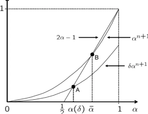
δ(αS)n+1− 2αS+ 1 = 0. (13)
On the equilibrium path, the reserve price in period t is given by αSβSvt−1∗ , where v∗t−1 = (αS)t−1.
Figure 2 illustrates the seller’s equilibrium strategy α. A point B is a solution of equation (13) for δ < 1 and a point B is a solution for δ = 1. As can be seen in Figure 2, there exists the maximum value ¯α < 1, and the equilibrium value α(δ) lies in the open interval (1/2, ¯α) depending on the discount factor δ ∈ (0, 1). The seller’s strategy α increases in δ and converges to the maximum value ¯α as δ → 1.
Before proceeding further with our analysis, we briefly consider hard close auctions. Since hard close auctions have only a first stage, each buyer does not have a chance to reply to other
Figure 2. The optimal decreasing rate of cutoff valuations A
B
buyers’ serious bids. McAfee and Vincent (1997) characterize the stationary linear PBE as follows.
Proposition 4. (McAfee and Vincent, 1997) In hard close auctions, there exists a unique stationary linear PBE (αH, βH) such that:
βH = 1 − δ n ·
1 − (αH)n
1 − δ(αH)n (14)
βH = 1 + 1 n
[(1 − δ) αH 1 − αH − 1
]. (15)
Combining these equations, we obtain:
δ(αH)n+1− 2αH + 1 = 0. (16)
On the equilibrium path, the reserve price in period t is given by αHβHvt−1∗ , where vt−1∗ = (αH)t−1.
6 Results
6.1 Theoretical implication
In this section, we compare the stationary linear PBE of soft close auctions and the stationary linear PBE of hard close auctions. Let (αS, βS) be the PBE of soft close auctions and (αH, βH) be the PBE of hard close auctions, respectively. By Proposition 3 and Proposition 4, we
immediately obtain αS= αH. The equality means that the rate of decrease in cutoff values is independent of the ending rules. In both auctions, the seller chooses a cutoff value vt∗ in period t such that every buyer i whose value satisfies vi≥ v∗t truthfully submits. The cutoff value v∗t is given by αvt−1∗ for t = 1, 2, · · · and v0∗ = 1. Because αS = αH, (vS∗)t = (vH∗)t for all t. We summarize this result as the following proposition.
Proposition 5. Let {(vS∗)t}∞t=1 be a sequence of cutoff values in a sequential soft close auc- tion and {(v∗H)t}∞t=1 be a sequence of cutoff values in a sequential hard close auction. In the stationary linear PBE, (v∗S)t= (vH∗ )t holds for all t.
Proposition 5 implies that both auction formats lead to the same allocation including the allocation period.
Despite the same allocation, reserve prices depend on the ending rules, because the buyer’s decision influences the reserve prices. Actually, an equilibrium reserve price is given by αβv∗t−1 in period t. The following theorem is the main result of this paper.
Theorem 1. Let {(rS)t}∞t=1be a sequence of reserve prices in soft close auctions and {(rH)t}∞t=1 be a sequence of reserve prices in hard close auctions, respectively. In the stationary linear PBE, (rS)t< (rH)tholds for all t.
The reserve prices in the hard close auction are greater than the reserve prices in the soft close auction in each period. Theorem 1 follows from βH > βS, which implies that the buyers are more likely to wait-and-see in the soft close auction than in the hard close auction.10 The intuition behind the theorem is that the buyers facing the soft close auction have the opportunity to submit bids after they observe the opponents’ bids; thus, they need not submit the bids in a hurry. In other words, the buyers in the soft close auction do not have any trade- off between submitting now and taking a wait-and-see attitude, while the buyers in the hard close auction do. The seller knows, of course, that the buyers in the soft close auction are more
10The result may seem contradict to the finding in Roth and Ockenfels (2002) and Ockenfels and Roth (2006) that buyers tend to bid earlier in the soft close auction than in the hard close auction. However, the difference comes from a difference of the situations analyzed. They consider the buyer’s bidding behavior within a single auction, while this paper considers that among auctions continuing sequentially.
likely to wait for lower reserve prices than in the hard close auction; thus, the seller rationally drops the reserve price to prevent her payoff from being discounted in the soft close auction. Thus, the seller chooses the lower reserve price in the soft close auction than in the hard close auction.
Finally, we consider the seller’s revenue. The same allocation in the both auction formats lead to the same revenue in each period; thus, the standard revenue equivalent theorem holds.
Theorem 2. In the stationary linear PBE, both ending rules lead to the same revenue, i.e. ΠS((vS∗)t|(v∗S)t−1) = ΠH((vH∗)t|(v∗H)t−1) holds for all t.
6.2 Comparison with the optimal auction
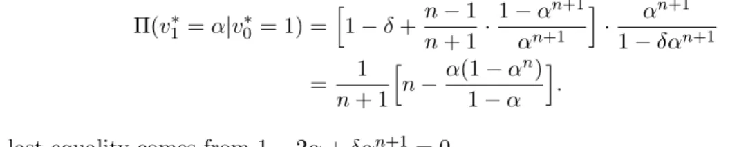
In period 1, the seller holds an initial belief that the highest value lies in [0, 1], and then the seller posts a cutoff value v1∗ = α. Under the uniform distribution F , in both auction formats, by using (15), the seller’s ex ante expected payoff is given by:
Π(v1∗= α|v∗0 = 1) =[1 − δ + n − 1 n + 1·
1 − αn+1 αn+1
]
· α
n+1
1 − δαn+1
= 1
n + 1 [
n −α(1 − α
n)
1 − α ]
. The last equality comes from 1 − 2α + δαn+1= 0.
Figure 3 shows a numerical example where δ = 0.99 and n = 10. In such a case, we obtain α = 0.500, βS = 0.631 and βH = 0.901. The seller chooses (rH)1 = 0.901 as a reserve price in period t = 1 in hard close auctions while (rS)1 = 0.631 in soft close auctions. The reserve prices in both auctions decrease at the rate α = 0.500. In this case, the seller’s expected payoff is calculated as Π(v1∗ = α|v∗0 = 1) = 0.8182.
On the other hand, in the optimal auction (Myerson (1981)), the seller should commit to the optimal reserve price given by (2) in period t. Under the uniform distribution F , the seller’s expected payoff is given by:
Π0(r0) = n − 1 n + 1+ (r0)
n− 2n n + 1(r0)
n+1
= n − 1 n + 1+
1 n + 1
( 1 2
)n
.
Figure 3. Reserve price in case of n=10 & Res. price r
Period t
Since r0 = 1/2, in a case of n = 10, the seller’s expected payoff is calculated as Π0(r0) = 0.8183. Therefore, due to the lack of commitment, the seller looses a little expected payoff.
In a case of δ = 0.99 and n = 2, we obtain α = 0.6153. The seller’s expected payoffs are given by:
Π(v1∗ = α|v∗0 = 1) = 0.3350, Π0(r0) = 0.4167.
In this case, the seller looses 20% of payoff due to the lack of commitment. 6.3 Data example
The difference between reserve prices according to ending rules is observed in Yahoo! Japan auctions. A seller sets a reserve price, which is called a starting price, at the beginning of an auction. Furthermore, Yahoo! Japan auctions allow each seller to freely select either a soft close or a hard close ending rule. The default rule is a hard close until 2008, while the default rule is a soft close since 2009. The data set consists of auctions in July 2008 and August 2008 (where the default rule is a hard close) and auctions in March 2011 (where the default rule is a soft close). Data were downloaded from each auction in the category “System” in “Nintendo DS” in “Toys”.11 12 The data are publicly obtained and freely downloaded during the auctions.
11The Nintendo DS is a dual-screen handheld game console developed and manufactured by Nintendo. It was released in 2004 in Canada, the United States, and Japan.
12Roth and Ockenfels (2002) and Ockenfels and Roth (2006) select the category Computers to analyze IPV auctions. Although the category Computers consists of a variety of items, this is unimportant because Roth and
For each auction, I recorded a starting price (reserve price), auction term (1 day - 8 days), a seller’s feedback number, a seller ID, an auction ID, a color of the item, and an ending rule.13 Although the qualities of the items auctioned may be distributed widely, we cannot verify the qualities. Some sellers note the quality by comments such as “The condition is good because I used it carefully” or reveal how long they used it; however, such information is not always credible.14 To standardize the qualities as much as possible; however, we exclude auctions selling the following items. (1) Broken items: these items are in other categories. The quality among items should be similar. (2) Bundled items: items with some softs or souvenirs are considered in other categories. Furthermore, we exclude items sold by auction stores because they sell many identical items; however, we are interested in sequential auctions with a single item. Yahoo! Japan auctions are equipped with many options.
The following three auctions were also excluded.15 (1) “Take-it-price” auctions in which the buyer can immediately buy the item by submitting a bid equal to a seller-defined take-it- price. Even though the hammer price may not reach the take-it-price, the item will be sold to a winner. (2) “Buy-it-now” auctions in which the starting price is posted as the buy-it-now price. If the buyer submits a bid equal to the buy-it-now price, then he immediately buys the item. and (3) “Secret reserve price” auctions were also excluded.
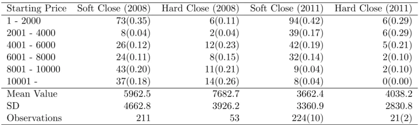
Table 1 show the distribution of reserve prices (fractions is provided in parentheses). As shown in Table 1, a mean value of starting prices in soft close auctions is lower than in hard close auctions, which is consistent with Theorem 1. However, we note that the difference is not statistically significant, because the distribution of starting prices in soft close auctions is not same as the distribution of starting prices in hard close auctions.
The data show that sellers prefer a soft close to a hard close, even though the theoretical
Ockenfels (2002) and Ockenfels and Roth (2006) focus not on the bidding time but the retail price. However, because we want to focus on the reserve price, items should be similar. Therefore, I selected the category
“System” in “Nintendo DS”.
13The feedback system for Yahoo! Japan auctions is similar to eBay’s. Buyers and sellers have the opportunity to give each other positive feedback (+1), neutral feedback (0) or negative feedback (-1). The positive feedback includes “Very good” and “Good”, and the negative feedback includes “Very bad” and “Bad”. The cumulative total of positive and negative feedback is what we call the “feedback number” for Yahoo! Japan auctions.
14See Jin and Kato (2006).
15In addition to the following auctions, we exclude new items in auctions between July 2008 and August 2008, because new items have a stable resale market in which they can be sold for close to list prices. However, the number of new items in auctions in March 2011 is quit a few (12 out of 246), hence we count both new items and secondhand items.
Table 1: Starting prices in Yahoo! Japan auctions
Starting Price Soft Close (2008) Hard Close (2008) Soft Close (2011) Hard Close (2011)
1 - 2000 73(0.35) 6(0.11) 94(0.42) 6(0.29)
2001 - 4000 8(0.04) 2(0.04) 39(0.17) 6(0.29)
4001 - 6000 26(0.12) 12(0.23) 42(0.19) 5(0.21)
6001 - 8000 24(0.11) 8(0.15) 32(0.14) 2(0.10)
8001 - 10000 43(0.20) 11(0.21) 9(0.04) 2(0.10)
10001 - 37(0.18) 14(0.26) 8(0.04) 0(0.00)
Mean Value 5962.5 7682.7 3662.4 4038.2
SD 4662.8 3926.2 3360.9 2830.8
Observations 211 53 224(10) 21(2)
result leads to revenue equivalence. Sellers select a soft close (211 prices) four times as many as a hard close (53 prices) in the data in 2008, and sellers select a soft close (224 prices) ten times as many as a hard close (21 prices) in the data in 2011. One possible reason is that sellers may think that a soft close can collect more potential buyers than a hard close due to extension of a deadline, results in higher revenues.
After the default ending rule changes from a hard close to a soft close, sellers are more likely to choose a soft close. The result may imply that, given the default soft close, choosing a hard close bears a strictly positive switching cost.
7 Conclusion
We developed a model of Internet auctions with a soft close, such as those used by Yahoo! Japan and Amazon. Our model captures the feature that all buyers can always submit bids even after observing other buyers’ bids. The buyers involved in the soft close auction face a weak trade-off between submitting in the current period and taking a wait-and-see attitude; thus, they are likely to wait for lower reserve prices in the future. Knowing the buyers’ incentives, the seller posts lower reserve prices in the soft close auction than in the hard close auction to prevent the seller’s expected payoff from being discounted. Although there exists a difference in reserve prices between the two auctions, the timing for selling is identical in the two auctions; thus, revenue equivalence holds for each period. This implies that the seller is indifferent between
choosing the two auctions given the number of the buyers. Also, the buyers are indifferent between choosing the two auctions given the number of the buyers. There is no selection bias for both the seller and buyers.
Naturally, we can extend the analysis to a common value assumption. Sequential auctions have not yet analyzed under a common value assumption, to my knowledge. The soft close auction may reveal more information about the buyers’ values than the hard close auction; thus, the seller may earn higher revenues in the soft close auction. If so, the seller is then likely to choose the soft close. This issue will be the future research.
References
[1] Ashenfelter, O. (1989), “How Auctions Work for Wine and Art,” Journal of Economic Perspectives 3, pp.23-36.
[2] Bajari, P. and Hortacsu, A. (2003), “The Winner’s Curse, Reserve Prices, and Endogenous Entry: Empirical Insights from eBay Auctions”, RAND Journal of Economics 34, No.2, pp.329-355.
[3] Caillaud, B. and Mezzetti, C. (2004), “How Auctions Work for Wine and Art,” Journal of Economic Perspectives 3, pp.23-36.
[4] Carey, K. (1993), “Reservation Price Announcement in Sealed Bid Auctions”, Journal of Industrial Economics, 41, No.4, pp.421-429.
[5] Cramton, P. C. (1984),“Bargaining with Incomplete Information: An Infinite Horizon Model with Continuous Uncertainty”, Review of Economic Studies 51, pp.579-594.
[6] Fudenberg, D., Levine, D. and Tirole, J. (1985), “Infinite-Horizon Models of Bargaining with One-Sided Incomplete Information”, in A. Roth (ed.), Game Theoretic Models of Bargaining, Cambridge: Cambridge University Press
[7] Grant, S., Kajii, A., Menezes, F. and Ryan, M. J. (2006),“Auctions with Options to Re- auction”, International Journal of Economic Theory 2, pp.17-39.
[8] Gul, F., Sonnecschein, H. and Wilson, R. (1986), “Foundations of Dynamic Monopoly and the Coase Conjecture”, Journal of Economic Theory 39, pp.155-190.
[9] Hoppe, T. (2008), “An Experimental Analysis of Parallel Multiple Auctions”, Faculty of Economics and Management Magdeburg (FEMM) Working Paper No.31.
[10] Jin, G.Z. and Kato, A. (2006),“Price, quality, and reputation: evidence from an online field experiment”, RAND Journal of Economics 37, No.4, pp.983-1005.
[11] Krishna, V. (2002), Auction Theory, Elsevier: Academic Press
[12] Lucking-Reiley, D. (2000),“Auctions on the Internet: What’s being Auctioned, and How?”, The Journal of Industrial Economics 48, No.3, pp.227-252.
[13] McAfee, R. P. and D. Vincent (1997),“Sequentially Optimal Auctions”, Games and Eco- nomic Behavior 18, pp.246-276.
[14] Milgrom, P. R. and R. J. Weber (1982),“A Theory of Auctions and Competitive Bidding, II”, in P. Klemperer (ed.), The Economic Theory of Auctions, Cheltenham, U.K.: Edward Elgar
[15] Myerson, R. (1981), “Optimal Auction Design”, Mathematics of Operations Research 6, pp.58-73.
[16] Ockenfels, A. and Roth, A. E. (2006),“Late and multiple bidding in second price Internet auctions: Theory and evidence concerning different rules for ending an auction”, Games and Economic behavior 55, pp.297-320.
[17] Riley, J. G. and W. F. Samuelson (1981),“Optimal Auctions”, American Economic Review 71, pp.381-392.
[18] Roth, A. E. and Ockenfels, A. (2002),“Last-minute Bidding and The Rules for Ending Second-price Auctions: Evidence from eBay and Amazon Auctions on the Internet”, Amer- ican Economic Review 92, pp.1093-1103.
[19] Samuelson, W. (1984), “Bargaining under Asymmetric Information”, Econometrica 52, pp.992-1005.
[20] Sobel, J. and Takahashi, I. (1983),“A Multistage Model of Bargaining”, Review of Eco- nomic Studies, 50, pp.411-426.
[21] Vincent, D. (1995), “Bidding off the Wall: Why Reserve Prices May Be Kept Secret?”, Journal of Economic Theory, 65, pp.575-584.
[22] Weber, R. (1983), “Multiple Object Auctions”, in R. Engelbrecht-Wiggans, M. Shubik, and R. Stark (eds.), Auctions, Bidding and Contracting: Uses and Theory, New York, NY.: New York University Press, pp.165-191.
8 Appendix
Proof of Lemma 1.
Proof. Suppose that a function β(·) determines a threshold v∗i = β(vi) for buyer i in a symmetric equilibrium. Fix a reserve price rtin period t, and consider a cutoff value v∗ such that β(v∗) = rt. We prove that all buyers with value v ≥ v∗ submits a serious bid b(vi) ≤ vi in a symmetric equilibrium.
Contrarily, suppose that b(vi) > vi for all i with value vi ≥ v∗. Because β(·) is a strictly increasing function, for vA, there exists vB such that vB < β(vA) < β(vB). Consider an expected payment of buyer j with value vj ∈ (vA, vB).
First, we consider a case of v(1)−j ∈ (vA, vj). If buyer j submits β(vj) according to an equilibrium strategy, the current price in the second stage is β(v(1)−j). Since it is a weakly dominant strategy for any buyer to submit his true value in the second stage, the buyer j’s payment is determined at β(v−j(1)). Consider a deviation for buyer j to submit β(vA) rather than β(vj). By using the deviation, the current price in the second stage is deter- mined as max{β(vA), β(v(2)−j)}; thus, the buyer j’s payment becomes max{β(vA), β(v(2)−j)}. Since max{β(vA), β(v−j(2))} < β(v−j(1)), the deviation is strictly profitable to the buyer j; a contradic- tion.
Second, we consider a case of v−j(1) < vA. In this case, both a bid β(vj) and a bid β(vA) lead to the same current price β(v(1)−j) in the second price, results in the same payment for the buyer j. Therefore, the deviation has no impact.
Finally, we consider a case of v(1)−j > vj. In this case, the buyer j does not win the auction; thus, the deviation has no impact.
Proof of Lemma 2.
Proof. Suppose that all buyers submit according to the truthful cutoff strategy in the first stage. We show that buyer i has no profitable deviation.
Fix a reserve price rt, and let vt∗ be a cutoff value such that β(vt∗) = rt.
First, we consider a case of vi < v∗t, where the buyer i does not submit a serious bid according to the truthful cutoff strategy. Possible deviations for the buyer i is to submit: a
serious bid b ≤ vi, and a serious bid b > vi. Suppose that the buyer i submits a serious bid b ≤ vi, leading to the second stage. Since the buyer i truthfully submits in the second stage, his expected payoff is given by:
viG(vi) −[rtG(rt) +
∫ vi
rt
ydG(y)].
Therefore, the buyer i cannot profitably deviate to submit a serious bid b ≤ vi since the following equation holds:
vt∗G(vt∗) −[rtG(rt) +
∫ v∗t
rt
ydG(y)]< δ(vt∗G(vt∗) −[rt+1G(rt+1) +
∫ v∗t
rt+1
ydG(y)]). Suppose next that the buyer i submits a serious bid b > vi. In this case, the buyer i cannot follow a dominant strategy in the second stage; thus, his expected payoff is lower than the above one. Therefore, the buyer i cannot profitably deviate to submit a serious bid b > vi.
Second, we consider a case of vi ≥ vt∗, where the buyer i truthfully submits a serious bid according to the truthful cutoff strategy. Suppose that the buyer i does not submit a serious bid. We separately consider two cases: no buyer submits a serious bid, and some buyers submit serious bids. No buyer submits a serious bid, meaning that the buyer i surely wins the auction in the next period; thus, the buyer i obtains the expected payoff given by:
δ(viG(vi) −[rt+1G(rt+1) +
∫ vi
rt+1
ydG(y)]).
Therefore, the buyer i cannot profitably deviate to wait and see since the following equation holds:
vt∗G(vt∗) −[rtG(rt) +
∫ v∗t
rt
ydG(y)]> δ(vt∗G(vt∗) −[rt+1G(rt+1) +
∫ v∗t
rt+1
ydG(y)]). The buyer i’s opponents’ serious bids induce the second stage, where all buyers truthfully submit; thus, the buyer i obtains the expected payoff given by:
viG(vi) −[rtG(rt) +
∫ vi
rt
ydG(y)]. Therefore, the buyer i cannot profitably deviate to wait and see.