Recent Advances in Empirical Analysis of Financial Markets:
Industrial Organization Meets Finance
∗Jakub Kastl†
June 2, 2016
Abstract
In this article I provide a selective review of recent empirical work in the intersection of finance and industrial organization. I describe an estimation method, which can be applied quite widely in financial and other markets where a researcher needs to recover agents’ beliefs. Using four applications I illustrate how combining this method with data from auctions and with a theoretical model can be used to answer various economic questions of interest. I start with the primary market for sovereign debt, focusing on treasury bill auctions of the US and Canada. I show how auction data together with standard tools from Industrial Organization can be used to shed light on issues involving market structure, market power and front-running. I continue by looking at the Main Refinancing Operations of the European Central Bank, the main channel of monetary policy implementation in the EURO-zone, and illustrate how auction data can be used to learn about typically opaque over-the-counter lending markets. I also discuss how to use these data indirectly to learn about dynamics of banks’ financial health and of their balance sheets. I then turn to the discussion of recent progress on estimation of systemic risk. I finish with thoughts on how to estimate a whole demand system for financial assets.
∗Thanks to Ali Horta¸csu for continued cooperation and to Ariel Pakes, Rob Porter, Azeem Shaikh and Moto Yogo for their comments. I am grateful for the financial support of the NSF (SES-1352305) and the Sloan Foundation. All remaining errors are mine.
1
Introduction
The last three decades marked a remarkable success in the development of tools in structural economic modeling, predominantly within the field of industrial organization. These techniques and tools can be applied more widely and the recent developments in health economics and to some extent in finance suggest that indeed there are many promising directions in which the literature can go. In this article I will talk about applying various tools from Industrial Organization to financial markets. The markets I will focus on here are (i) market for sovereign debt, and (ii) market for liquidity (short-term loans). I will argue that these and similar markets provide us with abundance of data and studying them can allow us to gain insights into many other areas of the economy. I will point out some open questions as I move through the applications.
The analysis of market power and market structure has been in spotlight of research in industrial organization (IO) since its early days. In finance, the market microstructure literature originates with Kyle (1985) and Kyle (1989). There are many papers that try to estimate the price impact of individual market participants based on Kyle’s model. Using a clever research design Shleifer (1986) shows that indeed demand curve for US equities seem to be downward sloping and thus there is potential for price-impact when large orders are executed. I will discuss in this paper how to try to assign this market power to individual market participants and how to quantify it.
In particular, since most countries, including the US and Canada, organize their primary market for debt around a few primary dealers, it is important to get a better understanding about the rents these primary dealers are accruing. Typically, these primary markets are organized as auctions. Since the number of primary dealers is typically fairly low, one may worry that their individual market power may cause prices (or yields) that clear the auction to be too low (too high). With the internet making it very easy to enter and participate in various remote markets, it may seem tempting to open up the auctions to new participants. Using data from treasury bill auctions I show how to evaluate market structure, how to quantify rents that primary dealers may be collecting from observing customers’ order flow, or how to evaluate the impact of entry of direct bidders in the US Treasury auctions. Since new entry might dissipate the rents the primary dealers enjoy, quantifying the effect of entry on primary market performance is a first order question.
above mentioned auctions of short-term loans. A bidder may obtain a loan from the auctioneer (a central bank) or he may approach a counterparty and negotiate terms privately. In equilibrium, the bidder should be indifferent between these two options and hence if one were able to observe the value of the bidder for a loan in the auction, one would equivalently be able to say what loan terms this bidder would have been able to obtain on the private market. Applying the IO tools allows us to estimate this value (or cost of alternatives financing) based on the observed bid and hence we will be able to gain insight into what terms a particular bank might have faced in the private market. Moreover, since these auctions are run at fairly high frequency (typically weekly), the dynamics of these funding costs might be an important source of information about issues like bank health. I will also show how this dynamics may be used to study systemic risk.
While introducing the applications, I describe an estimation method, which can be used quite widely in financial and other markets. The basic idea is that an economic model provides a link between the primitives of interest and observables which is based on some equilibrium relationship. Since this equilibrium relationship typically depends on agents’ beliefs about rivals’ strategies, the described method involves simulating these beliefs using a resampling strategy.
Finally, in the last section I briefly lay out two ways how to one can go about estimating a full demand system for financial assets, which are viewed as differentiated products. The first is based on a product-space demand model building on Deaton and Muellbauer (1980). The second, which may substantially reduce the number of parameters and also allows for evaluating welfare from introduction of new goods, is based on the characteristics space demand model developed in Berry, Levinsohn and Pakes (1995).
One caveat to have in mind while reading this paper is that with the recent antitrust case involving LIBOR fixing and ongoing investigation of bankers due to manipulation of other key reference interest rates (EURIBOR, TIBOR), we should be aware of possible collusion which would typically alter the key relationship between the observable data and objects of interest. Various models of collusion available in the IO literature might be used to address this issue, but I will leave the discussion of collusion for future surveys.1
2
Using Auction Data
To begin, in this section I review the workhorse model, variants of which will be utilized in the applications. Readers not interested in technical details of the theoretical model and estimation can skip this section. However, the description of the estimation algorithm and the discussion of the general ideas underlying it may be useful in many other applications. The data examined in the applications described later as well as data in many other settings are generated from strategic behavior of agents participating in various environments that can be described as games. Here we will talk mostly about auctions, but in many other environments the games that the agents
1
play might be different: they might be choosing prices or quantities, designing products, choosing whether and which markets to market etc. The important takeaway from the following discussion is that typically the variables or parameters of interest will be related to observables via some equilibrium relationship, which involves players’ beliefs about rivals’ strategies (and possibly beliefs about the distribution of some aggregate uncertainty) at the time the game is played. One of the goals of this section is to describe an estimation method that will allow for recovering these beliefs from the observed data. The second goal is to develop a general theoretical model through which the observed data will be linked to unobservables of interest.
The common feature of auctions in financial markets examined below is that they involve a one-time sale of large quantities of homogeneous good: Treasury Bills, Bonds, Notes, or short-term loans. It is convenient and without much loss to abstract from the discreteness of the quantities demanded as the quantities requested are typically quite large. Instead, it is useful to express bidders’ demands in terms of the share of the total supply. Treating the quantity domain as a connected set allows for convenient and elegant analysis of equilibrium bidding behavior, which also clearly reveals the intuitive relationship between an oligopoly pricing problem and a uniform price auction.
Virtually for any auction mechanism, we can express the equilibrium bid as willingness-to-pay minus a shading factor:
BID =W T P −SHADIN G. (1)
2.1 Theoretical Model
I begin with the basic share auction model that is based on Wilson (1979). Since in most real-world auctions strategies that bidders may employ are restricted to take form of step functions, Wilson’s original model should be modified to incorporate these restrictions as in Kastl (2012) before taking it to the data. I start with the basic symmetric model with private information and private values and will introduce its variants and various generalizations when discussing the applications later. Unlike Kyle (1989), Vives (2011), Rostek and Weretka (2012) or Ausubel et al. (2014) who obtain closed from solutions for equilibrium demands after imposing appropriate assumptions on utilities and uncertainty distributions, we will work here under less restrictive assumptions. Let us assume
there are N potential bidders at the cost of obtaining only implicit equilibrium characterization
via a set of necessary conditions. Each bidder is endowed with (possibly multidimensional) private signal,Si, which affects the underlying value of the auctioned goods.
Assumption 1 Bidders signals,S0, S1, ..., SN, are drawn from a common support[0,1]M according
to an atomless joint d.f. F(S0, S1, ..., SN) with density f.
For the characterization results below some conditions on the smoothness of the distribution
of residual supplies is needed. This can come either from properties of F(·) or one can assume
uncertain continuously distributed supply as is common in electricity auctions (and which will also be required for consistency of one of the proposed estimators). I will for simplicity assume that there is exogenous uncertainty about the supply, Q.
Assumption 2 Supply Qis a random variable distributed on Q, Q with strictly positive density conditional onSi ∀i.
Obtaining a share q of the supply Q is valued according to a marginal valuation function
vi(q, Si). We will impose following conditions on this function.
Assumption 3 vi(q, Si) is non-negative, measurable and bounded, strictly increasing in each
com-ponent of Si ∀q, and weakly decreasing and continuous inq ∀Si.
Note that under Assumption 3, values are assumed to be private since vi(·) does not depend
on private information of the rivals. Since in many settings (and particularly in financial markets)
we may worry that values are interdependent and marginal value of bidder i might depend on
signal of bidderj, it is important to provide more discussion of this assumption. I will provide this discussion while discussing one of the applications in Section 3.4.1 below.
specify the marginal quantity, qk−qk−1, that a bidder is biddingbk for. I will also allow a bid l,
which is sure to lose, and hence basically corresponds to not participating in the auction.
Assumption 4 Each playeri= 1, ..., N has an action set:
Ai =
(
~b, ~q, Ki
: dim~b= dim (~q) =Ki∈ {1, ..., K},
bik∈B ={l} ∪
0,¯b, qik∈[0,1], bik > bik+1, qik < qik+1 )
.
Finally, I will assume that rationing is pro-rata on the margin. This means that if demand at the market clearing price were to exceed the supply, all bidders’ bids submitted exactly at that price would be adjusted proportionally.
I will use the term K-step equilibrium to refer to a Bayesian Nash Equilibrium of the auction game where the bidders are restricted to use at mostK steps. In other words, a K-step equilibrium is a profile of strategies, such that each strategy is a step function with at most K steps and it maximizes the expected payoff for (almost) every type si for all i.
2.1.1 Discriminatory Auction
I begin with laying out the equilibrium of a discriminatory auction: an auction in which every bidder has to pay his bid for all units he/she wins. LetVi(q, Si) denote the gross utility: Vi(q, Si) = Rq
0 vi(u, Si)du. The expected utility of a bidderiof typesi who is employing a strategyyi(·|si) in
a discriminatory auction given that other bidders are using{yj(·|·)}j6=i can be written as:
EU(si) =
Ki
X
k=1
[Pr (bik> Pc> bik+1|si)V (qik, si)−Pr (bik> Pc|si)bik(qik−qik−1)] (2)
+ Ki
X
k=1
Pr (bik=Pc|si)EQ,s−i|si[V (Q
c
i(Q,S,y(·|S)), si)−bik(Qci(Q,S,y(·|S))−qik−1)|bik=Pc]
where I let qi0 = biKi+1 = 0. The random variable Q
c
i(Q,S,y(·|S)) is the (market clearing)
quantity bidder i obtains if the state (bidders’ private information and the supply quantity) is
(Q,S) and bidders submit bids specified in the vectory(·|S) = [y1(·|S1), ..., yN(·|SN)]. Pc is the
(random) market clearing price.
A Bayesian Nash Equilibrium in this setting is a collection of functions such that (almost)
every type si of bidder i is choosing his bid function so as to maximize his expected utility:
yi(·|si) ∈ arg maxEUi(si) for a.e. si and all bidders i. The system of necessary conditions
Proposition 1 Under assumptions 1-4 in any K-step Equilibrium of a discriminatory auction, for almost all si, every step k < Ki in the equilibrium bid function yi(·|si) has to satisfy
Pr (bik > Pc > bik+1|si) [v(qik, si)−bik] = Pr (bik+1≥Pc|si) (bik−bik+1) (3)
and at the last step Ki it has to satisfy v(q, si) =biKi where q = supq,s−iQ
c
i(q, s−i, si,y(·|S)).
Note that this condition is simply a multi-unit counterpart of the equilibrium condition for bidding in a first-price auction: g(b) (v−b) =G(b), where G(b) is the CDF (and g(b) is the PDF) of the distribution of the first order statistic of rival bids (i.e., of the highest of rival bids) (see Guerre, Perrigne and Vuong (2000)). The trade-off in the multiunit environment remains virtually the same. The bidder is simply trading off the expected surplus on the marginal (infinitessimal) unit versus the probability of winning it.
Condition (3) provides us with a mapping from observables (bids) to the object of interest: the willingness-to-pay v(q, si) in the spirit of the general equation (1). The estimation approach is
similar in spirit to Laffont and Vuong (1996) and Guerre et al. (2000) and has been proposed for the multiunit auction environment first by Horta¸csu (2002). Note that (3) is simply a necessary condition for an optimal choice ofqk. The set of these conditions (one for eachk) thus identifiesK
points of the function v(q, si). The optimality condition with respect to the bidbk can be derived
in a straightforward manner by differentiating (2), but it cannot be simplified and interpreted as naturally as equation (3). Nevertheless, it may allow a researcher to obtain tighter bounds on the functionv(q, si). McAdams (2008) discusses identification of the primitives using other restrictions
in more detail.
The question of equilibrium existence in the environment where bidders bid using step func-tions has been addressed in Kastl (2012). Proposition 2 in that paper establishes existence of an equilibrium in distributional strategies for a discriminatory auction with private values and supply uncertainty whenever the potential dependence between private signals is not “too large.” Formally, it is required that the probability measure associated with the distribution function F(S1, ..., SN)
is absolutely continuous with respect to QNi=1µi whereµi is the marginal ofµ on Si. For the case
of symmetrically informed bidders, but uncertain supply, Pycia and Woodward (2015) show that there is a unique pure-strategy Baysian-Nash equilibrium.
2.1.2 Uniform Price Auction
Turning to the uniform price auction, the expected utility of a bidderiwho is employing a strategy
yi(·|si) given that other bidders are using{yj(·|·)}j6=i can be written as:
EUi(si) = EQ,S−i|Si=siu(si, S−i)
= EQ,S−i|Si=si
"Z Qc
i(Q,S,y(·|S))
0
where as before Qci(Q,S,y(·|S)) is the (market clearing) quantity bidder i obtains if the state
(bidders’ private information and the supply quantity) is (Q,S) and bidders bid according to
strategies specified in the vector y(·|S) = [y1(·|S1), ..., yN(·|SN)], and similarly Pc(Q,S,y(·|S))
is the market clearing price associated with state (Q,S).
Once again, the system of necessary conditions implicitly characterizing a BNE in this environ-ment is the link between the observables and unobservables that we seek to establish. Kastl (2011) provides the following characterization result linking the bids and the underlying marginal values.
Proposition 2 Under assumptions 1-4 in anyK-step equilibrium of a Uniform Price Auction, for almost all si, every step k in the equilibrium bid function yi(·|si) has to satisfy:
(i) Ifv(qik, si)> bik
Pr (bik > Pc > bik+1|si) [v(qik, si)−E(Pc|bik > Pc > bik+1, si)] =qik
∂E(PcI[b
ik≥Pc ≥bik+1]|si)
∂qik
(4)
(ii) Ifv(qik, si)≤bik
Pr (bik> Pc> bik+1|si) [v(qik, si)−E(Pc|bik> Pc> bik+1, si)] + (5)
+ Pr ((bik=Pc∨bik+1=Pc|si) ∧ T ie)E
(v(Qc, si)−Pc)∂Q
c
∂qik|(bik=P c
∨bik+1=Pc) ∧ T ie, si
=qik∂E(P c
I[bik≥Pc≥bik+1]|si)
∂qik .
A technical detail that arises in the model with discrete bidding is that when bidding above her marginal valuation for some units, we can no longer be sure that a tie does not occur with positive probability in equilibrium. The cost of shading the demand captured on the LHS of (5) now also includes the effect on the surplus at the expected quantity after rationing in the event of a tie.
Equations (3), (4) and (5) are the counterparts of equation (1) for the specific auction models we will be discussing below. I will now move on to describing how to estimate the “SHADING” term in each case.
Equilibrium of a uniform price auction where bidders use step functions is more subtle as ties may occur in equilibrium with positive probability. Existence (in fact existence of a pure strategy equilibrium in non-decreasing strategies) obtains for the limiting case of no restriction on the number of steps as results from McAdams (2006) can be applied. With the restriction on the
number of steps, one can only provide existence results for an ε-equilibrium. See Section 3.1.1
2.2 Estimation
The estimation approach described in what follows can be generalized to many other settings than just auctions. The main point is that the relationship between observables (bids in case of an auction, submitted student preferences in case of school matching mechanisms, buy-sell orders in case of data from equity markets etc) and objects of interest, i.e., preferences, valuations or willingness-to-pay, is given by an equilibrium relationship of an explicit economic model, in which each participant’s behavior depends on his/her beliefs about rivals’ behavior. Typically the researcher assumes a Nash Equilibrium (or its appropriate form such as a Bayesian Nash Equilibrium or a refinement such as a Perfect Bayesian Equilibrium when selection is necessary) which then restricts participants beliefs about rivals’ play to be consistent with the actual strategies. In many environments or games, the equilibrium strategies depend on the rivals’ actions only indirectly, the actual uncertainty is about some functional of these actions. For example, in the applications discussed here, the uncertainty is about where the market will clear, i.e., about the market clearing price. In case of school choice, the uncertainty is about whether a given school might have an open spot for the applicant. In case of equity markets, the uncertainty might be about whether a counterparty for a particular trade can be found. One way to account for this uncertainty in estimation non-parametrically is to assume that all participants agree on its distribution and hence any differences in their observed strategies are due to differences in their private information. In that case, one can account for the uncertainty about the object of interest and thus estimate its probability distribution by “resampling,” i.e., by following a bootstrap-like procedure where by drawing repeated samples of strategies (by sampling with replacement from the observed data) one simulates different possible states of the world and thus eventually obtains an estimate of the distribution of the random variable(s) of interest. This idea appeared originally in Horta¸csu (2002) and was later applied in Horta¸csu and McAdams (2010) and Kastl (2011). Such an estimator is a particular form of a V-statistic, which has useful implications for characterizing its asymptotic behavior. It should be intuitive to see that as one constructs more and more samples (as the data set gets larger and thus the observed strategies span more and more of the type space), one obtains more and more simulated states of the world, where the probability of a type profile being in some subset of the type space [0,1]M×Q, Qcorresponds to the probability of that subset implied by the population distribution functions given in Assumptions 1 and 2. I will now describe this approach in the context of auctions in detail.
2.2.1 Typical Data Set
A typical auction data set {B1t, ..., BN t, Qt, Xt}Tt=1, consists of of T auctions and for each t, the
set of bids B1t, ..., BN t, the realized supply, Qt, and some auction covariates, Xt, where N is the
number of (potential) bidders. In the auctions we will talk about here, Bit is typically a function
for) into the bid, typically specified in terms of yield. In most applications, bit(·) takes form of
the step function, {(qitk, bitk)}Kk=1it where Kit number of steps bidder i uses in auction t. Supply
may be deterministic and announced by the auctioneer prior to the auction (as is the case with US Treasury auctions) or may be stochastic since the auctioneer may adjust the preannounced quantity later (as is the case with the ECB auctions of short-term loans). In some applications, bidders might be of different types, which may either be observable or latent. For example, we might have primary dealers and other bidders and we may have a good reason to believe that the underlying distribution of their willingness-to-pay may differ across these groups. We may therefore have C bidder classes, and thus haveNct potential bidders of classc in auctiont.
2.2.2 Estimating the Distribution of the Market Clearing Price
Examining equations (3) and (4), it is clear that to establish a link between the observed bids and the object of interest, v(·), one needs to estimate the distribution ofPc. With such an estimate in hand, one can utilize the usual plug-in approach of Guerre et al. (2000) and obtain an estimate of
v(·). The distribution of Pc from perspective of a bidder with signal si is defined as
H(X)≡Pr (X≥Pc|si) =E{Q,Sj6=i}}I
Q−X j6=i
y(X|Sj)≥y(X|si)
(6)
where I(·) is the indicator function and E{·} is an expectation over the random supply and other bidders’ private information. Essentially, this equation states that the probability that the market clearing price will be lower thanXis equal to the probability that the set of types and the realization of the supply are such that the aggregate demand of those types falls short of the supply. Horta¸csu and Kastl (2012) show that one can estimate H(·) by first defining an indicator of excess supply at priceX (given bid functions {yj(X|sj)}j6=i and i’s own bid yi(X|si)) as follows:
Φ{yj(X|sj)}j6=i;X
=I
Q−X j6=i
yj(X|sj)≥yi(X|si)
An estimator ofH(X) is based on a V-statistic, which is based on all subsamples (with replace-ment) of size (N−1) from the full sample ofN T datapoints:
ξFˆ;X, hT
= 1
(N T)(N−1)
(T,N) X α1=(1,1)
...
(T,N) X αN−1=(1,1)
Φ yα1, ..., yαN−1, X
(7)
where αi ∈ {(1,1),(1,2), ...(1, N), ...,(T, N)} is the index of the bid in the subsample and ˆF is
It is straightforward to see that an estimator defined as a simulator of ξFˆ;X, hT
by drawing
only M subsamples rather than all (N T)(N−1) is consistent as T → ∞ (and under appropriate
conditions on the rate at which the number of simulations, M, increases - see Pakes and Pollard
(1989) for more details). Cassola, Horta¸csu and Kastl (2013) establish that it is also consistent as
N → ∞ provided some further technical conditions are satisfied. This latter result is particularly important when studying financial markets and auctions in general (but also in other applications), since it allows to use data from one auction at a time and thereby keep constant many unobserv-able characteristics. When the economic environment is changing and it is hard to capture these changes through covariates so that pooling data across auctions might be dubious, proceeding with estimation within an auction might be the preferred way to go. Horta¸csu and Kastl (2012) further show how to modify this estimator in order to allow for asymmetries and the presence of covari-ates by introducing weighting into the resampling procedure which is similar to a nonparametric regression.
Applying the estimation approach described above, we can thus obtain an estimate of the “Shading” factor in (1) that determines the wedge between the submitted bid and the actual willingness-to-pay. With an estimate of bidder’s actual willingness-to-pay, which is of course ulti-mately equivalent to having an estimate of that bidder’s demand curve, we can start evaluating that bidder’s market power, which leads naturally to our first application.
3
Market Power and Market Structure in Treasury Securities
3.1 US Bond, Notes and Treasury Bill Auctions
To begin our discussion of applications of the previously described theory and estimation procedure, I start by focusing on one of the most important financial markets in the world: the market for US Debt Instruments (treasury bills, notes and bonds). In 2013 alone, the US Treasury auctioned $7.9 trillion of debt. In 2007, the net interest amounted to $238 billion and represented 8.7% of Government expenditures. The average daily trading volume exceed $565 billion that same year (the global equity trading was under $420 billion daily at that time). In mid 2008, there was $4.6 trillion in outstanding marketable debt, which was approximately a quarter of the US credit markets. Based on its size, it is clear that this is one of the most important financial markets in the world.
3.1.1 Market Rules
(sealed) bids, currently via an electronic interface, and the market clearing price is determined as the highest price (or lowest yield) at which there is no excess supply, ie at which demand equals supply. There are two types of bids that bidders may submit: (i) noncompetitive (up to a limit of $5 million), whereby a bidder guarantees himself an allocation of the requested amount at whatever the market clearing price will be and (ii) competitive, in which both the price and quantity can be freely specified. The market for new issuance of debt has been historically organized around a fairly small number of “primary dealers.” In addition to primary dealers, there are also other participants in the treasury auctions: the direct and indirect bidders. Direct bidders, as the name suggests, participate on their own behalf (own trading accounts). As we will see below, these become more and more important in the treasury auctions since they purchase larger share over time. The indirect bidders are customers placing bids through a primary dealer. It is important to point out that some of these customers are very large players in the treasury markets themselves: various asset managers or large pension funds that simply choose not to participate directly. This list of customers may also include Foreign monetary authorities placing their bids through the New York Fed. One question we will address here is the extent to which observing such customer order flow contributes to PDs’ profits.
3.1.2 Primary Dealer System
The PD system started in 1960 with 18 PDs, grew to 46 PDs by 1988 and declined again to the current 22 PDs. To be a primary dealer (as currently governed by the Primary Dealers Act of 1988), a bank or securities broker/dealer must commit to active participation in security auctions (i.e., to submit “reasonable bids” for a fraction of at least N1P D of the announced supply, whereNP D is the number of primary dealers. Primary dealers are also required to make bids when the Fed conducts open market operations and to report on their activity to the Fed’s open market trading desk. There are, however, also many important benefits. For example, during the implementation of the Quantitative Easing (QE) program, only PDs were allowed to participate. Also, and perhaps more importantly, as mentioned above primary dealers act as intermediaries at the primary market: they submit bids on behalf of their clients who choose not to participate directly.
3.2 Market Power and Uniform Price Auction
When talking about market power, typically we have in mind a situation where a profit maximizing firm chooses price (or output) such that it exceeds (falls short of) the competitive price (quantity), i.e., p(q)> C′(q). In IO many researchers such as Bresnahan (1989), Porter (1983), Ellison (1994) or Genesove and Mullin (1998) estimated the extent of market power by introducing a parameter,
cost and the market power parameterθ.2
Let us recall for the moment the equation for optimal pricing by a monopolist that faces an uncertain demand (satisfying appropriate regularity conditions):
Ep+Ep′(q)q=c′(q) (8)
Rewriting this equation as
Ep=c′(q)−θEp′(q)q (9)
where (loosely speaking) θ ∈ [0,1] is a parameter indexing market power. For θ = 0 we have
perfect competition and forθ= 1 we have a monopoly. Since the early days of the New Empirical
Industrial Organization, parameter θ was one of the central objects of interest. Assuming some
behavioral model (such as Nash Equilibrium in prices), and given some useful variation in the data, this parameter can be estimated in a fairly straightforward manner.
Let us rewrite (4) as
E(Pc|bk> Pc > bk+1)
| {z }
BID BY A PRICETAKER
= v(qk) | {z }
WTP
− qk
Pr (bk> Pc> bk+1)
∂E(Pc;bk ≥Pc≥bk+1)
∂qk
| {z }
MARKET POWER (SHADING)
(10)
Comparing (9) and (10) it seems natural to estimate the extent of market power of individual bidders in a uniform price auction by evaluating the last term (10). The goal here is not to estimateθas in (9, but rather to evaluate the importance of the last term in (10) and study how it varies across bidders and/or auctions. In the context of treasury auctions, in the next subsection we will be interested whether the shading factor of primary dealers differs from that of other market participants.
3.3 Market Structure in the US Treasury Auctions
3.3.1 Bidding Data and Market Overview
Horta¸csu, Kastl and Zhang (2015) analyze the detailed bidding data from July 2009 - Oct 2013. The securities in their sample range from 4 week bills to 10 year notes, with 822 auctions of 4-week, 13-week, 26-week, 52-week bills and cash management bills, and 153 auctions of 2-year, 5-year, and 10-year notes. The total volume of issuance through these auctions was 27.3 trillion US dollars, with the average issue size around 28 billion dollars. While anonymized, these data differentiate bidders by three classes: primary dealers, direct bidders and indirect bidders. The measures of market concentration typically employed in anti-trust or IO literature such as HHI or C4 are not alarmingly high in this market (HHI is 561 for bills and 450 for notes and bonds). Nevertheless,
we may worry that primary dealers may be able to significantly leverage their market power in this market - especially since they get to observe the customers’ order flow. Primary dealers are, as a class of bidders, the largest purchasers of primary issuances. In terms of tendered quantities, primary dealer tenders comprise 69% to 88% of overall tendered quantities. Direct bidders tender 6% to 13% and Indirect bidders 6% to 18% of the tenders. In terms of actual purchases (or quantities awarded), the PDs obtain about 63% of the auction volume. Nevertheless, the share of direct bidders is rising over the past few years. There are several natural questions to ask with these data. First, we may want to verify that the message that the concentration measures tell (i.e., that the market seems fairly competitive) is indeed supported by the data. Second, we may be interested in digging deeper into the primary dealer system and try to quantify the rents that primary dealers enjoy due to observing their customers’ bids before submitting their own.
To look at the first question, Horta¸csu et al. (2015) begin with investigating the bids directly. Table 3 in that paper summarizes how quantity-weighted bids compare to a US Treasury published benchmark yield on the day of the auction. Indirect bidders systematically bid lower yields than the market-level prevailing yield (and substantially so in auctions of 6-month Tbills), the direct bidders bid around the prevailing yields and the primary dealers bid on average above these yields. Of course these numbers per se are hard to interpret, since there might be other effects at play that are not visible when looking just at the quantity-weighted bids. For example, if primary dealers need to absorb much larger amounts of the auctioned instruments (recall that they have to bid for
1
NP D share of the supply), they will need to be compensated for this and hence their bids might
reflect this compensation even in absence of any market power or direct price effect considerations. Table 4 investigates the differentials in bid yields through regressions of the following form:
bqwit =αg+βQit+ξt+εit (11)
where bqwit is the quantity-weighted average yield bid submitted by bidder iin auction t,αg is the
intercept corresponding to group g (i.e., primary dealers, direct bidders and indirect bidders), Qit
is the total (or maximal) quantity demanded by i in auction t expressed as a share of the total
issuance,ξt are auction fixed effects, andεis the usual regression error term. The table illustrates
the results separately for Treasury Bills (short-term maturities) and Treasury Notes (long-term), as it is possible that the market dynamics are very different across these different classes of securities. Since the regressions also include auction fixed effects, they provide within-auction comparisons that account for differing supply-demand conditions that affect the level of the bids.
bidders demanding larger quantity may have higher demand for the security, but they may also have higher market power. The regressions indicate that larger bidders systematically bid higher yields. The effect is quite large – the coefficient estimate indicates that a size increase of 10% of total issue size accounts for 1(6) basis point increase in the bid yield.
While accounting for bidder size appears to lower the differences in bid yields across bidder classes, Primary Dealers still appear to bid higher yields than Direct and Indirects even accounting for their offer share of the total issue.
As noted above, since bids reflect both differences in demand and also differences in market power, it is difficult to interpret these documented differences in bids. Even though larger bidders bid higher yields (i.e., lower prices), this is not prima facie evidence that large bidders exercise market power; it is possible that larger bidders also have lower willingness-to-pay. This is where the model comes in - to allow the researcher to decompose these effects.
3.3.2 Modification of the Model of Bidding
We now need to modify the model of bidding introduced earlier in order to separate out the market power and demand components of bid heterogeneity so that we explicitly incorporate that the three groups of bidders (primary dealers, and direct and indirect bidders) may potentially be ex-ante heterogeneous. As mentioned previously, the model, and the measurement it will allow us to conduct, willrely on the assumption of bidder optimization. In essence, what we will end up doing is to measure the elasticity of (expected) residual supply faced by each bidder. This is directly observable in the data, and does not require behavioral assumptions. This elasticity will be our measure of the “potential market power” possessed by each bidder. Assuming that bidders are expected profit maximizers who will exercise their market power in a unilateral, noncooperative fashion, we can then estimate the willingness-to-pay/demand that rationalizes the observed bid. In order to do that I modify Assumption 1 as follows:
Assumption 1′ Direct and indirect bidders’ and dealers’ private signals are independent and drawn from a common support [0,1]M according to atomless distribution functions FP(.), FI(.), and FD(.) with strictly positive densities.
Similarly, Assumption 3 is replaced by one allowing for heterogeneous valuation function:
bill market, and in that context private values cannot be rejected. Note that under this assump-tion, the additional information that a primary dealerj possesses due to observing her customers’ orders,ZjP, simply consists of those submitted orders. As will become clear below, this extra piece of information allows the primary dealer to update her beliefs about the competitiveness of the auction, or, somewhat more precisely, the distribution of the market clearing price. I will come back to this issue when discussing the application quantifying the value of the order flow.
Let us now define the probability distribution of the market clearing price from the perspective of a direct bidderj, who is preparing to make a bidyD(p|sj). The probability distribution of the
market clearing price from the perspective of direct bidder j will be:
Pr (p≥Pc|sj) =E{S
k∈D∪P∪I\j,Zl∈P}I
Q− X
m∈P
yP(p|Sm, Zm)−X l∈I
yI(p|Sj)− X k∈D\j
yD(p|Sk)≥yD(p|sj)
(12)
where E{·} is an expectation over all other bidders’ (including indirect bidders, primary dealers, and other direct bidders) private information, and I(·) is the indicator function.
This appears to be a complicated expression, but it essentially says that the probability that
the market clearing price Pc will be below a given price level p is the same as the probability
that residual supply of the security at price p will be higher than the quantity demanded by
bidder j at that price. In the expression inside the indicator is the residual supply function faced
by bidder j. This residual supply function is uncertain from the perspective of the bidder, but
its distribution is pinned down by the assumption that the bidder knows the distribution of its competitors’ private information and the equilibrium strategies they employ. This assumption is also what makes the estimation technique based on resampling the observed strategies to simulate the perceived uncertainty work.
For a primary dealer, the distribution of the market clearing price is slightly different, since the dealer will condition on whatever information is observed in the indirect bidders’ bids. In a (conditionally) independent private values environment, this information does not affect the primary dealer’s own valuation, or her inference about other bidders’ valuations. The distribution of the market clearing price from the perspective of primary dealerj, who observes the bids submitted by indirect biddersm in an index setM|, is given by:
Pr (p≥Pc|sj, zj) =
E
Sk∈I\M|,Sl∈D,Sn∈P\jZn∈P\j|zj
I
RS(Q, p)≥y P
(p|sj, zj) + X
m∈M|
yI(p|sm)
(13)
where RSp, Q, ~S, ~Z = Q −Pk∈I\M
|y I(p|S
k) −Pl∈DyD(p|Sl)−Pn∈P\jyP(p|Sn, Zn), i.e.,
the residual supply at price p given supply realization Q and realization of private information
~
S, ~Z. Note that the main difference in this equation compared to equation (12) is that the
the dealer “learns about competition” – the primary dealer’s expectations about the distribution of the market clearing price are altered once she observes a customer’s bid.
Finally, the distribution of Pc from the perspective of an indirect bidder is very similar to a direct bidder, but with the additional twist that the indirect bidder recognizes that her bid will be
observed by a primary dealer, m, and can condition on the information that she provides to this
dealer. The distribution of the market clearing price from the perspective of an indirect bidderj,
who submits her bid through a primary dealerm is given by:
Pr (p≥Pc|sj) =
E{S
k∈I\j,Sl∈D,Sn∈PZn∈P|sj}I
Q− X
k∈I\j
yI(p|Sk)− X
l∈D
yD(p|Sl)− X
n∈P
yP(p|Sn, Zn)≥yI(p|sj)
(14)
whereyI(p|s
j)∈Zm.
Note that the probability distributions from perspective of a direct bidder or uninformed pri-mary dealer, or that of an informed pripri-mary dealer (given his/her observation of customer order flow) and that of an indirect bidder can then be estimated using equations (12), (13) and (14) using the resampling technique described above. With the estimates of the probability distributions of market clearing price in hand, we can use equation (10) to estimate the willingness-to-pay (or, equivalently, the shading factor) at every observed bid. it is also worth pointing out the connection with the Kyle model (Kyle 1985). In Kyle’s model there is an informed trader and uninformed liquidity traders and a market maker. In our current model, market participants can be heteroge-neous in terms of their information sets and hence their price impact (or what is typically called in the context of Kyle-style models lambda) is also different.
Given equation (10) a natural definition of shading is as follows.
Definition 1 The average shading factor is defined as: S(θi) =
PKi
k=1qk[vi(qk,θi)−E(P c|b
k>Pc>bk+1,θi)] PKi
k=1qk
.
This is a quantity-weighted measure of shading, where shading at stepkis defined as the difference between the marginal value, vi(qk, θi) and the expected market clearing price, conditional on kth
step being marginal, E(Pc|bk> Pc > bk+1, θi). Another way to interpret this shading factor is to
note that it corresponds to the weighted sum of the second term on the right-hand side of equation (10), which is essentially the expected inverse elasticity of the residual supply curve faced by the bidder - the object of interest in general studies of market power in IO.
zero to 10% market share allows a dealer to shade her bids by 0.3 basis points. Lastly, the authors report that there are larger differentials in shading for Notes than for Bills, albeit the qualitative findings remain the same.
Putting the previous findings together, the results suggest that, under the assumption of ex-pected profit maximization, the main reason why Primary Dealers bid higher yields than other bidder groups is not because they have lower valuation for the securities, but because they are able to exercise more market power: the size of their demands and their information about customer order flow allows them to leverage their impact on the market clearing price by “shading” their bids more.
3.3.3 Quantifying Bidder Surplus
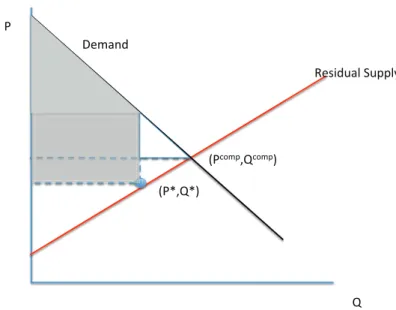
A question related to bid-shading that we can answer through the estimates obtained thus far is to quantify how much infra-marginal surplus bidders are getting from participating in these auctions. To compute ex-post surplus, we first obtain point estimates of the “rationalizing” marginal valuation functionv(q, s) at the (observed) quantities that the bidders request as described above. We then compute the area under the upper envelope of the inframarginal portion of the marginal valuation function, and subtract the payment made by each bidder. To compute ex-ante (or rather interim) surplus, one can integrate the ex-post surpluses over the distribution of the market clearing prices. I should provide here abundant caution regarding what “infra-marginal bidder surplus” means. Any counterfactual auction system would also have to allow bidders to retain some surplus. Indeed, in Figure 1, we see very clearly that even if bidders bid perfectly competitively, i.e. reveal their true marginal valuations without any bid shading, they would gain some surplus from the auction, just because they have downward sloping demand curves. Indeed, if there are any costs of participating in the auction, it would have to be justified by the expected surplus. In terms of assessing the cost effectiveness of the issuance mechanism, the most we can say is that the bidder surplus under an efficient allocation reflects a conservative upper bound to the amount of cost-saving that can be induced by a change in issuance mechanism.
!"
#" $%&'()*+",)--+." /%0*1("
2!34#35"
2!670-4#670-5" /%0*1("
Figure 1: Illustration of Bid Shading when Residual Supply is Known
formats. Using auctions run by the Receiver General, the fiscal agent of the Canadian federal government, Chapman, McAdams and Paarsch (2007) use bounds to argue that surpluses bidders enjoy in the discriminatory auctions of term deposits are tiny. While in all these examples there are rents that accrue to the participants due to some market power they enjoy (ie the residual supplies faced by these participants are not completely flat), it seems that these rents are very small, especially if one were to take into account the typical cost of employing a number of skilled people to run a trading desk.
An interesting question for further research is evaluating the impact of competition on these rents. Elsinger, Schmidt-Dengler and Zulehner (2015) analyze the Austrian treasury auctions and, in particular, investigate the impact of competition on bidders’ surpluses. They argue that evaluating the surpluses using a model similar to the one used here leads to them finding a smaller effect of competition on surplus than would be the case using a simple reduce-form measures.
when-issued or resale markets. Aggregating the surpluses over the entire set of auctions in their data set (which amounted to about $27 trillion in issue size), Direct and Indirect Bidders’ aggregate surplus is estimated to be about $1.6 billion, or about 0.6 basis points in terms of the annualized yield. Primary Dealers’ infra-marginal surplus, however, appears to be significantly larger. For Primary Dealers, the derived surplus might not necessarily be in line with the differentials with the quoted secondary market prices of these securities. Primary Dealers’ demand is typically quite large, and fulfilling such levels of demand is likely to have a price impact in the secondary markets. Moreover, retaining Primary Dealership status has a number of complementary value streams attached to it beyond the profits derived from reselling the new issues. For example, being a Primary Dealer allows firms access to open market operations and, especially in this period, the QE auction mechanism that is exclusive to primary dealerships. Between March 2008 and February 2010, Primary Dealers also had access to a special credit facility from the Fed to help alleviate liquidity constraints during the crisis. Quantifying these costs and benefits to being a primary dealer is an interesting avenue for future research.
Horta¸csu et al. (2015) report that Primary Dealers derive most of their infra-marginal surplus from the longer end (2 to 10 year notes) of the maturity spectrum. There may be a number of reasons why demand for this part of the maturity spectrum is more heterogeneous across bidders. One possibility is the presence of different portfolio needs across dealers’ clientele. Moreover, there are typically alternative uses for such securities beyond simple buy-and-hold – Duffie (1996) shows that this part of the spectrum can be particularly valuable for its use as collateral in repo transactions. Surpluses derived from the shorter end of the maturity spectrum, which may have fewer alternative uses, are much smaller. Overall, Horta¸csu et al. (2015) find that Primary Dealers’ derived surplus aggregated to $6.3 billion during their sample period. Compared against the $27 trillion in issuance, Primary Dealer surplus makes up for 2.3 basis points of the issuance. Along with the Direct Bidder and Indirect Bidder surpluses, bidder surplus added up to 3 basis points during this period. Once again, I should emphasize that any other issuance mechanism would have to provide bidders with surpluses to ensure participation and to reward them for their private information. Moreover, even if bidders are behaving in a perfectly competitive manner, without displaying any bid-shading, they would enjoy surpluses. However, we can conservatively estimate that revenue gains from further optimizing the issuance mechanism are bounded above by 3 basis points.
as another control variable. This variable serves a rough proxy for the order-flow information that the Primary Dealer is privy to. Indeed, the regression reveals a significant correlation between the number of Indirect Bidders who routed their bids through a Primary Dealer, and the surplus (controlling for the bidder’s size). An additional Indirect Bidder going through a Primary Dealer would be correlated with about seven thousand dollars more in surplus for Bills and $200K gain in Primary Dealer surplus for Notes. Since Primary Dealers on average route 2.5 Indirect Bids in Notes auctions, this estimate suggests that we can ascribe about $500K or about 25% of their surplus in Notes auctions to information contained in Indirect bids. However, it should be noted that there are important caveats to interpreting this as the “value of order flow.” It is possible that Primary Dealers who observe more Indirect bids may have systematically higher valuations for the securities, and hence may be getting higher surpluses due to this.
To estimate the value of order flow more convincingly, one would like to have a data set that would reveal a primary dealer’s bid both before the customers’ orders arrive and his/her updated bid after customers’ bids arrive. Since the US Treasury data only contains final bids, it is not well suited to answering this question. In the section we turn to the next application where I will describe the analysis of Canadian Treasury auctions, which will provide us with an opportunity to quantify the value of customers’ order flow and also to address the important question of what it is that primary dealers might be learning about when observing customers’ bids.
3.4 Value of Customer Order Flow
Horta¸csu and Kastl (2012) analyze data from Canadian treasury auctions, which are similar to the data from US Treasury auctions described in the previous section. The data set contains all indi-vidual bids submitted in these auctions. Canadian treasuries are sold via discriminatory auctions, hence the link between the data and the objects of interest, the willingness-to-pay measures, is provided by equation (2). As previously mentioned, a unique feature of the Canadian data set is that it contains timestamps of individual bids and the researcher can thus observe if and how bids change within an auction as the deadline approaches. In particular, primary dealers frequently submit bids only to subsequently being asked to submit bids on behalf of a client. Since orders of large clients, such as pension funds, are tracked separately by the Canadian Treasury, the times-tamps reveal when such bids arrived and oftentimes the primary dealer subsequently decides to revise his/her original bid. Horta¸csu and Kastl (2012) build a simple model that rationalizes why a primary dealer might want to submit a bid before customers’ orders arrive - basically introduc-ing uncertainty in whether customers’ bids arrive at all and if they do, whether the subsequently updated dealer bid will make it in time to make the deadline.
information in their bids. There may be reasons for customers to voluntarily share their information with dealers as well. For example, Bloomberg Business published an article on 4/4/2013 where a representative of Blackrock, the world’s largest asset manager, described why Blackrock chooses to
participate indirectly by submitting bids through PDs: “While we can go direct, most of the time
we don’t. We feel that the dealers provide us with a lot of services. Our philosophy at this point is, to the extent we can share some of that information with trusted partners who won’t misuse that information, we prefer to reward the primary dealers that provide us all that value.”3 In previous work studying the Canadian treasury market, Horta¸csu and Sareen (2006) find that some dealers’ modifications to their own bids in response to these late customer bids narrowly missed the bid submission deadline, and that such missed bid modification opportunities had a negative impact on dealers’ ex-post profits.
With slight modifications on top of our auction model from Section 2.1 that allow for customers and primary dealers submitting bids in various times, we can use equation (2) and the method described in Section 2.2 to estimate willingness-to-pay that would rationalize each observed bid. With these estimates in hand, it is natural to proceed by comparing expected profits corresponding to a primary dealer’s bid that was submitted absent any customer’s order information to expected profits corresponding to the bid that was submitted after observing customer’s order (both within the same auction). While intuitive, this approach would be premature. In Assumption 3, we have imposed that bidders’ values are private - in particular, we assumed that if a primary dealer were to learn a customer’s signal by observing that customer’s bid, she would not update her estimate of the value. This assumption is often questioned and treasury bills are often mentioned as an example of objects that should be modeled using a model with interdependent values. Given the data available in the Canadian treasury auctions, we can formally test this assumption, at least as far interdependency of values between primary dealers and their customers is concerned.
3.4.1 Private versus Interdependent Values in Treasury Bill Auctions
Recall that in the Canadian Treasury Bill auctions the researcher observes instances where a bidder (primary dealer) submits two bids in the same auction, one before customer’s order arrives and one after it arrives. This setting thus provides us with a natural laboratory where to investigate whether primary dealers are just learning about competition in the upcoming auction (and not updating their valuation estimates) or whether the PDs may also be learning about fundamentals, and hence update their value estimates after observing customers’ bids. When deciding how to translate willingness-to-pay into the bid, the primary dealer must form beliefs about the distribution of the market clearing price (as equation (2) reveals). To form such beliefs, the primary dealer integrates over all uncertainty: the signals of rival primary dealers, the signals of all customers, which primary dealer a customer might route her bid through etc. By observing a customer’s order, part of this
3
uncertainty gets resolved: a primary dealer can therefore update her belief about the distribution of the market clearing price by evaluating (13). Since this updating can be easily replicated in the estimation by appropriately adapting the resampling technique, it allows us to form a formal hypothesis test about whether values are indeed private. In particular, letvBIk (qk, θ)
K
k=1 denote
the vector of the estimated willingness-to-pay that rationalizes the observed vector of bids before the customer’s order arrives (hence, “BI”),bBIk (qk, θ)
K k=1, and
vkAI(qk, θ) KBI
k=1 denote the vector
of the estimated willingness-to-pay that rationalizes the observed vector of bids after the customer’s bid arrives (hence, “AI”),bAIk (qk, θ)
KAI
k=1. If we were to observe a bid for the same quantity being
part of both the bid before customer’s information arrive and the bid after its arrival, we can simply formulate a statistical test at that quantity. Let Tj(q) = vBI(q, θ)−vAI(q, θ) be the difference
between the rationalizing willingness-to-pay for a given quantity, q, before and after information arrives (taking into account the updating about the distribution of the market clearing price during the estimation). Testing the null hypothesis (of no learning about fundamentals) then involves testing that Tj(q) = 0,∀j, q. Of course, the null hypothesis is essentially a composite hypothesis of
all modeling assumptions (e.g., in addition to private values, we also assume independence etc.). To test the hypotheses jointly, since there is no result on uniformly most powerful test, we can define several joint hypotheses tests and perform them concurrently. For example, the following test is motivated by the well-knownχ2-test, which can be additionally standardized by the standard deviation of the asymptotic distribution of each individual test statistic.
T =
(N,T) X (i,t)=(1,1)
Ti,t(q)2 (15)
Horta¸csu and Kastl (2012) report that the null hypothesis of no learning about fundamentals from customer’s bids can be rejected neither based on (15), nor based on several alternative tests. While this still does not preclude interdependency of values between primary dealers themselves, given that many of the customers are large players (such as Blackrock) this evidence is at least suggestive that modeling information structure in treasury auctions as private values is reasonable. It is important to note that the crucial point about the information structure is not that the security of interest might have common unknown value at the secondary market after the auction, but rather whether or not the primary dealers have different information about this ex-post valuebefore the auction. If the information is symmetric, and potentially imperfect, the heterogeneity in values (and thus in bids) might still be attributable purely to heterogeneity in the private component of the values.
3.4.2 Quantifying Order Flow
the dynamics of bidding within an auctions is particularly useful for two reasons: First, since the bidding takes place typically within few minutes before the auctions deadline, it is quite reasonable to assume that nothing else is changing other than primary dealer’s getting (or not) information about customers’ orders. In language of empirical industrial organization, this allows the researcher to control unobserved heterogeneity at a very fine level: one needs to rely neither on variation across auctions, nor across bidders within an auction. This, therefore, allows the researcher to quantify the value of order flow by calculating the expected surplus (profits) of a primary dealer associated with the original bid (before customers’ order information arrives) and compare it to the expected profits associated with a bid after the customer’s information arrives. Of course, in doing so, one has to take into account that the beliefs about the distribution of the market clearing price will change when customers’ order arrives as can be clearly seen by comparing equations (12) and (13). With these two distributions, in hand we can now estimate not only ex-post profits (given the realized demands of other primary dealers and other customers), but also the ex-ante profits given the appropriate distribution of the market clearing price. Horta¸csu and Kastl (2012) report that about one third of PDs’ profits can be attributed to the customers’ order flow information. Overall, however, the auctions seem fairly competitive and the profits thus do not seem excessive - recall that Horta¸csu et al. (2015) reached a similar conclusion for the US Treasury auctions.
The main takeaway from the Canadian treasury auctions is thus that (i) customers’ order flow is an important source of primary dealers’ rents (up to one third in the Canadian auctions) and (ii) private values may be a reasonable approximation of the information structure in treasury bill auctions.
Another important question is why indirect bidders voluntarily choose to submit their bids through a primary dealer rather than to participate in the treasury auctions directly. This is an excellent direction for future research. For example, the quote from a Blackrock executive mentioned in footnote 3 above suggests that there might complementary services that PDs are providing to the indirect bidders. One example might be helping them to execute a large trade in an asset that otherwise quite illiquid, but there may be many others. Building a theory of these complementarities and quantifying their value would be an excellent research question to pursue.
3.5 Extracting Information about Bank’s Balance Sheets and their Over-the-Counter Trading Opportunities
In this section I want to focus on a different kind of auctions, the Main Refinancing Operations (MRO) of the European Central Bank (ECB), analyzed in Cassola et al. (2013). MROs are the main tool of monetary policy implementation at ECB’s disposal. Basically, these are discriminatory auctions of short-term (typically 1-weekl) repo loans.4 Banks participate by offering bids for loans
4
at various yields and of various sizes. The loans are collateralized, but the quality requirements for collateral are typically much weaker than those in the private transactions. By varying the minimum bid rate (minimum yield) and the total available supply, the ECB is trying to target the overnight unsecured interest rate (EONIA) in the financial markets. There are four key facts about the raw data at the onset of the financial crisis in mid- to late 2007. First, the spreads between secured and unsecured interest rates (even short-term) diverged substantially starting in August 2007 for all maturities. Second, bids in the MROs became “more aggressive” - in the sense that the submitted yields became higher. Third, bids became quite dispersed suggesting an increased heterogeneity in demand (either within or across banks). Fourth, some and in few instances in fact most if not all banks submitted bids that exceeded the published EURIBOR (Euro Interbank Offer Rate) for loans with the same maturity, where bids are for collateralized loans whereas EURIBOR is supposed to represent the rate for an unsecured loan. This is clearly evidence that most if not all banks would not be able to secure funding at the EURIBOR
One important question to address is, therefore, whether the increased heterogeneity in bids is due to an increased heterogeneity in willingness-to-pay or whether the heterogeneity in bids could also be masking the strategic effect: some banks might simply be changing their bids in response to other banks’ changing their bidding behavior rather than changes in their underlying willingness-to-pay.
There are two main goals of the analysis. The first goal is to illustrate that in order to interpret the bidding data in a meaningful way, one needs an economic model such as the one in Section 2.1. The reason is that the bids are strategic choice variables that the participants (banks) submit taking the strategic environment, i.e., the auction game being played, into account. This implies that one needs a model to decompose the changes in bids into those caused by changes the underlying objects of interest, such as the willingness-to-pay for a loan, and those caused by changes in the strategic environment. As before, I will proceed in a sequence of steps. First, I will illustrate that a natural interpretation of a bank’s willingness-to-pay for a loan in the MROs is the cost of funding of that bank in that week. Second, I will talk about how the time series variation of these funding costs can be used to draw inference about dynamics of banks’ balance sheets and hence to distinguish “healthy” banks and those that might be getting into financial difficulties.
3.5.1 Willingness-to-Pay and Funding Costs
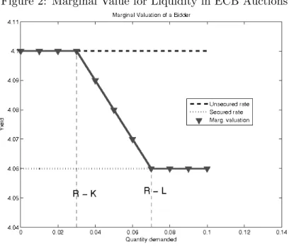
In Assumption 3 I imposed some structure on the willingness-to-pay as one of the primitives of our model, but at this point it is worthwhile to discuss where this object may be coming from. Due to the substitutable nature of ECB and interbank loans, these demand functions are very much dependent on a bank’s outside funding opportunities. Figure 2 depicts the willingness-to-pay function v(q, si) for some realization of the private signal si. In this figure, I assume that the
consider the following stylized model in which bankihas a liquidity need (possibly due to a reserve requirement, to improve its balance sheet, or to close a funding gap) of Rit at time t. This must
be fulfilled through three alternative channels: (i) a loan from the ECB, (ii) unsecured interbank lending, which is done through over-the-counter deals, or (iii) secured interbank lending, which is also done over-the-counter. These channels are substitutes, but access to them is limited based on collateral availability. In particular, assume that bank i has Lit units of liquid (high-quality)
collateral acceptable by secured interbank lending counterparties. The bank also has KitLit units
of securities that are acceptable by the ECB and perhaps also by other counterparties as collateral, but are either subject to “haircuts.” The haircuts applied to this set of securities effectively increase the interest rate at which the bank can borrow against these securities; these rates are bounded below by the “secured” interbank lending rate, sit, that the bank faces, and bounded above by the
“unsecured” interbank lending rate, uit , which requires no collateral. The bank’s
willingness-to-pay for the rstRit−Kit euros of funding, thus, is equal to its unsecured funding rate,uit. Between
the Rit−Kit and Rit−Lit, , the bank faces different haircut rates depending on its portfolio of
securities it can post as collateral. The lastLiteuros of funding can be obtained from the “secured”
interbank market.
Figure 2: Marginal Value for Liquidity in ECB Auctions
participate in these auctions. A researcher can, therefore, recover a panel of funding costs: for each bank that participates, one recovers a rationalizing willingness-to-pay in a given week, which corresponds to the best alternative of funding for that bank. On the the other hand, this next-best alternative depends on the quality of that bank’s available collateral and on its credibility or perceived riskiness. This suggests that looking at the dynamics of these funding costs can be informative about individual banks’ financial health.
3.5.2 Dynamics of Banks’ Balance Sheets
Having obtained a time series of funding costs for each bank, we can ask whether there are signif-icant patterns over time, and in particular during the onset of the financial crisis. Cassola et al. (2013) report (Table III and Figure 6) that for about two thirds of banks the funding costs indeed significantly increased, albeit for many of those banks this increase was not too big. However, there were few banks for whom the funding costs increased quite substantially - up to 66 basis points (in terms of the annualized yield), which is quite substantial given the short-term maturity of the loans.
3.5.3 Separating the Strategic Effect
As mentioned above, in order to meaningfully interpret the observed changes in bids, one needs to take into account the strategic effect. Cassola et al. (2013) provide a useful illustration of this important point. Figure 7 in Cassola et al. (2013) shows the bid distributions separately for banks that are identified as suffering relatively more from the financial crisis, in the sense that these banks’ funding costs significantly increased during the early period of the crisis, and banks whose funding costs remained relatively unaffected by the crisis. While the two distributions are different, they have very similar means and virtually overlapping supports. Nevertheless, Figure 8 illustrates that the two distributions of willingness-to-pay (or funding costs) are quite different across the two groups. Naturally, the distribution of funding costs of the group of banks that were affected more by the crisis dominates that of the other group in the sense of first order stochastic dominance.
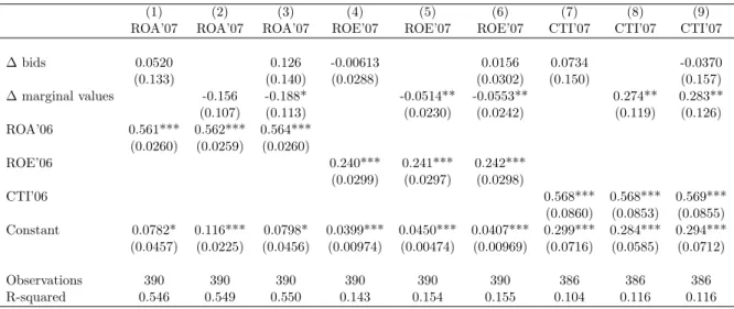
Perhaps more importantly, Table 1 illustrates this point further. The table depicts regressions of various performance measures taken from the balance sheets data on changes in bids, changes in funding costs or both. The regressions are of the following form:
Pi,2007 =β0+β1∆bqwi +β2∆vqwi +β3Pi,2006+εi (16)
where Pi,t is the value of an accounting performance measure in firm iand year t, a change ∆bqwi
Table 1: Correlation between bank performance ratios and marginal values/bids
(1) (2) (3) (4) (5) (6) (7) (8) (9) ROA’07 ROA’07 ROA’07 ROE’07 ROE’07 ROE’07 CTI’07 CTI’07 CTI’07
∆ bids 0.0520 0.126 -0.00613 0.0156 0.0734 -0.0370 (0.133) (0.140) (0.0288) (0.0302) (0.150) (0.157) ∆ marginal values -0.156 -0.188* -0.0514** -0.0553** 0.274** 0.283** (0.107) (0.113) (0.0230) (0.0242) (0.119) (0.126) ROA’06 0.561*** 0.562*** 0.564***
(0.0260) (0.0259) (0.0260)
ROE’06 0.240*** 0.241*** 0.242*** (0.0299) (0.0297) (0.0298)
CTI’06 0.568*** 0.568*** 0.569*** (0.0860) (0.0853) (0.0855) Constant 0.0782* 0.116*** 0.0798* 0.0399*** 0.0450*** 0.0407*** 0.299*** 0.284*** 0.294*** (0.0457) (0.0225) (0.0456) (0.00974) (0.00474) (0.00969) (0.0716) (0.0585) (0.0712)
Observations 390 390 390 390 390 390 386 386 386 R-squared 0.546 0.549 0.550 0.143 0.154 0.155 0.104 0.116 0.116
The dependent variables in this table are bank performance ratios (ROA, ROE, and CTI) reported year-end 2007. The independent variables are the pre- vs. post-crisis (Aug. 9, 2007) change in a bank’s quantity-weighted average price bids (∆ bids) and estimated marginal valuations (∆ marginal values).
We also control for the year-end 2006 performance ratios. Standard errors are in parentheses, with (***) indicating p<0.01, (**) p<0.05, and (*) p<0.1.
the performance measures. Banks whose funding costs increase suffer a larger drop in Return-on-Assets (or Return-on-Equity) or their Cost-to-Income ratio worsens. Perhaps surprisingly, similar correlations do not appear when one uses the bids directly, i.e., before “purging” them of the strategic effect. Such divergence in results would be impossible in a single-unit auction since a bid is a monotone function of value. There are two reasons for which such difference may arise in this environment. First, in multiunit auctions we may not have a monotone equilibrium. More plausibly though, some aggregation occurs before the regressions are run: bids and values are multidimensional objects - they are step functions - and they are aggregated to one-dimensional statistics by taking a quantity-weighted average and then a difference is taken between two such averages (pre and post crisis). This aggregation may thus also upset the monotonicity. In any case, Table 1 illustrates that taking the strategic effect out from the bids is a necessary step to obtain the quantities of interest. While we may find some of the assumptions underlying the model of equilibrium bidding behavior questionable or unsatisfactory, the model still delivers estimates that pass an out-of-sample test presented in this table.