JIMF13 Recent site activity Mototsugu Shintani

Exchange rate pass-through and in

_fl

ation: A nonlinear time

series analysis

Mototsugu Shintani

a,*

_{, Akiko Terada-Hagiwara}

b

_{, Tomoyoshi Yabu}

c

a_{Department of Economics, Vanderbilt University, Nashville, TN 37235, USA} b

Economics and Research Department, Asian Development Bank, Mandaluyong City 1550, Manila, Philippines c_{Faculty of Business and Commerce, Keio University, Minato-ku, Tokyo 108-8345, Japan}

JEL Classification: C22

E31 F31

Keywords: Import prices Inflation indexation Pricing-to-market

Smooth transition autoregressive models Sticky prices

a b s t r a c t

This paper investigates the relationship between the exchange rate pass-through (ERPT) and inflation by estimating a nonlinear time series model. Based on a simple theoretical model of ERPT deter-mination, we show that the dynamics of ERPT can be well approximated by a class of smooth transition autoregressive (STAR) models using the past inflation rate as a transition variable. We employ several U-shaped transition functions in the estimation of the time-varying ERPT to US domestic prices. The estimation result suggests that declines in the ERPT during the 1980s and 1990s are associated with lowered inflation.

_{2012 Elsevier Ltd. All rights reserved.}

1. Introduction

Within the framework of new open economy macroeconomic models, the degree of exchange rate pass-through (ERPT) into domestic prices is one of the key elements in evaluating international spill-over effects of monetary policy. Over the past decade, a number of empirical studies have investigated whether ERPT, defined as the response of domestic inflation rates to the changes in exchange rates (or

*Corresponding author. Tel.:þ1 615 322 2196; fax:þ1 615 343 8495.

E-mail addresses:[email protected](M. Shintani),[email protected](A. Terada-Hagiwara),tomoyoshi. [email protected](T. Yabu).

Contents lists available atSciVerse ScienceDirect

Journal of International Money

and Finance

j o u r n a l h o m e p a g e : w w w . e l s e v i e r . c o m / l o c a t e / j i m f

in marginal costs), decreased during the 1980s and 1990s.1If there was a reduction in ERPT, it is natural to conjecture some interaction between the ERPT and the inflation rate because the timing corre-sponds, in many countries, to a period of low and stable in_flation. This view is emphasized byTaylor (2000), who states that “the lower pass-through should not be taken as exogenous to the infl a-tionary environment (p.1390).”

The purpose of this paper is to investigate Taylor’s hypothesis on the positive relationship between the ERPT and inflation by estimating a nonlinear time series model. In particular, we employ the class of smooth transition autoregressive (STAR) models so that the degree of ERPT to domestic prices can be determined by the lagged domestic inflation rate. Most previous empirical studies on the positive association between ERPT and inflation focus on the cross-country evidence, including the analyses by

Calvo and Reinhart (2002), Choudhri and Hakura (2006), andDevereux and Yetman (2010). This paper differs from the existing studies in that we examine the role of inflation in the time-varying ERPT under the time series modeling framework.

In the empirical literature on the nonlinear adjustment of real exchange rates, STAR models have been popularly employed in many studies, includingMichael et al. (1997), Taylor and Peel (2000), Taylor et al. (2001), andKilian and Taylor (2003), among others. However, STAR models have rarely been used in analyses of the ERPT.2While nonlinear mean reversion of real exchange rates implies the full ERPT in the long-run, it does not imply the time-varying ERPT. We employ several U-shaped transition functions in STAR models to consider alternative forms of time-varying ERPT. Our method is applied to monthly US import and domestic price data and evaluatesfluctuations of ERPT during the period from 1975 to 2007.

To motivate our nonlinear regression approach, wefirst present a simple theoretical model of importingfirms where the ERPT becomes a nonlinear function of the past inflation rate. Our model is closely related to a model of ERPT developed byDevereux and Yetman (2010)so that the optimal price level depends directly on the nominal exchange rate, which corresponds to the marginal cost, and that importing _firms endogenously select the probability of adjusting their price to an optimal level. However, our model differs from their model in several aspects. First, for every period, a fraction of

firms make afinite-periodTaylor (1980)type staggered contract of an inflation indexation rule. Second, each_firm faces the problem of opting out of a contract. When_firms opt out, they can set an optimal price by paying afixed cost. Because the ERPT increases if morefirms set an optimal price, and the probability of opting out depends on the past inflation rate, our model predicts that ERPT depends on the lagged inflation. This prediction is in contrast to the case ofDevereux and Yetman (2010)where the ERPT depends on the steady-state inflation level of the economy. We show that the dynamics of ERPT predicted by the theoretical model can be well approximated by the STAR structure, and that the past decline during the 1980s and 1990s and the recent increase in the ERPT to US prices are well explained by the STAR model.

The remainder of the paper is organized as follows. Section “Theoretical motivation” briefly describes the prediction from the theoretical model. Section“Econometric procedures”introduces the empirical model. Estimation results are provided in the section “Empirical results”, followed by “Conclusions”in the next section.

2. Theoretical motivation

In this section, we briefly describe our theoretical model of importingfirms, which predicts that the ERPT depends on the lagged in_flation.3The basic setup is similar toDevereux and Yetman (2010)in that importingfirms are monopolistic competitors who import differentiated intermediate goods from abroad. A representative domesticfinal good producer purchases all the imported intermediate goods

1 _{See, for example,Goldberg and Knetter (1997), Otani et al. (2003), Campa and Goldberg (2005), Sekine (2006) and} McCarthy (2007).

2 _{One of the few exceptions is a study of UK import prices byHerzberg et al. (2003). However, their study did not} find supporting evidence on nonlinearity.

3 _{The details of the model are provided in theAppendix.}

and combines them to produce afinal output. Pricing contracts between the importers and thefinal good producer are valid forN(2) periods long, and a constant fraction 1/Nof all importingfirms write their contracts in any given time period. However,_firms are allowed to opt out during the contract period and to deviate from the contract pricing rule by paying afixed costF(>0). During thefirstN*(1) periods of the contract,firms follow the contract pricing rule and fully index their prices to aggregate in_flation

p

tof the initial contract period. Iffirms opt out of the contract afterN* periods, for the

remaining periods of the contractN N*, they can charge the desired price^p_{t ¼}stþptþ

m

wherestis

the nominal exchange rate,p

t is the foreign currency price and

m

is a mark-up. Since the marginal cost stþptis assumed to follow a random walk process (with the variance of its increment

s

2), all thefirms

entering into new contracts at timetset their price atp^_t. Therefore, forfirms that write their contracts

at time t and opt out at time t_þN*, the entire price path is given by

f^pt;^ptþ

p

t;._;^_{ptþ ðN 1Þ}

_p

_t;^_pt

þN;.;p^tþðN 1Þg.

We follow Ball et al. (1988), Romer (1990), and Devereux and Yetman (2002, 2010), among others, and re-formulate thefirm’s optimization behavior so that the probability of (not) changing its price to the desired price level is endogenously determined. Let

k

ðtÞ_{be the (conditional)} prob-ability that a_firm under contract in the current period will maintain the contract price in the next period. Here, a superscriptt in parenthesis signifies that this probability applies to all the firms entering into new contracts at timet, but not to firms in other cohorts. After setting the new contract price att, the firms observe the aggregate inflation

p

t and choose

k

ðtÞ to minimize the

expected loss function given by

Lt ¼Et 2

4 X N 1

j¼1

bk

ðtÞj_^p

tþj

p

t ^ptþj 2

3

5 þ

1

k

ðtÞ

k

ðtÞ

X N 1

j¼1

bk

ðtÞj XN j

[_¼1

b

[ 1

!

F (1)

where

b

is a discount factor. The above function implies that the loss is an increasing function of the inflation rate in absolute value. As the inflation rate rises (relative to the size of thefixed cost), thefirm can minimize loss by avoiding the inflation indexation. This strategy leads to a lower

k

ðtÞ_{(or a shorter} average length ofN*). In an extreme case of a high inflation,

k

ðtÞ _{¼0 (orN}*

¼1) is selected with a pricing path given byfp^t;^ptþ1;.;p^tþðN 1Þg. In the other extreme case of a low inflation,

k

ðtÞ¼1

(orN*_¼N) can be selected with a pricing path given by_f^p_t;p^_tþ

p

t;p^tþ2

p

t;._;p^_{tþ ð}N 1_Þ

p

_tg. In general, between the two extreme cases, the solution becomes a function of the inflation rate and can be expressed as

k

ðtÞ _¼

_k

_ð

_p

_tÞ.

The (short-run) ERPT is de_fined as the_first derivative of

p

twith respect to a change in marginal cost,

D

_ðstþptÞ. Using the dynamic Phillips curve derived from the model, the ERPT can be expressed in

terms of

k

ðt jÞ _¼

_k

_ð

_p

t jÞforj ¼1;.;N 1, so that the ERPT depends directly on the lagged inflation.

WhenN¼2, the model reduces to the two-periodTaylor (1980)model with a possibility of opting out in the second period as considered byBall and Mankiw (1994)andDevereux and Siu (2007). In this simple case, the inflation dynamics follow a nonlinear AR(2) model with the ERPT given by 1

k

_ð

p

_t 1Þ=2 where

k

ð

p

t 1Þ ¼ 1fj

p

t 1j

ffiffiffiffiffiffiffiffiffiffiffiffiffiffi

F

s

2

p

g.Fig. 1shows the predicted relationship between the lagged inflation rate and the ERPT. Abrupt transitions at the threshold values ffiffiffiffiffiffiffiffiffiffiffiffiffiffi

F

s

2

p

and ffiffiffiffiffiffiffiffiffiffiffiffiffiffi

F

s

2

p

suggest the possibility of approximating the ERPT by a variant of a threshold autoregressive (TAR) model, which is sometimes referred to as the three-regime TAR model or the band TAR model. WhenN becomes greater than 2, transitions become smoother. For example, whenN_¼3, inflation follows a nonlinear AR(3) model with the ERPT given by 1 _f

k

_ð

p

t 1Þ þ

k

ð

p

t 2Þ2g=3 where

k

ð

pt

Þ ¼

F

s

2

_p

2

t

2

b

F 2

s

2 ₄

_p

2 t ;

provided F

s

2

_p

2

t >0 and ðF

s

2

p

2tÞ þ2

b

ðF 2

s

2 4

p

2tÞ<0. As shown in Fig. 2 (which

imposes

b

= 0.98 and

p

t 1 ¼

p

t 2), the smooth nonlinear relationship between the inflation and the

ERPT resembles the adjustment dynamics described by a class of STAR models with a U-shaped transition function using the lagged inflation rate as a transition variable.

3. Econometric procedures

This section introduces the nonlinear time series model that we will use in the empirical analysis. There are three main predictions of the theoretical model on the ERPT we wish to incorporate in the empirical model. First, higher in_flation (in absolute value) results in a higher degree of the ERPT. Second, the ERPT may be expressed as a symmetric function of the past inflation rates around zero. Finally, in general, the dynamics of the ERPT can be described as a smooth rather than an abrupt transition using the past in_flation rate as the transition variable possibly with multiple lags. The only exception is a special case of two-period contract that predicts a discrete transition typically assumed in the TAR model.

To incorporate these features in a parsimonious parametric model, we primarily employ the exponential STAR (ESTAR) model, where a symmetric U-shaped transition function is represented by an exponential function

G_ðzt;

g

Þ ¼ 1 exp n

g

z2_to;

0.0 0.2 0.4 0.6 0.8 1.0

-10.0 -5.0 0.0 5.0 10.0

t-1)

ERPT

Fig. 2.ERPT and inflation: three-period contract case (N¼3). Solid line:F¼260 ands2_{¼170. Dotted line:F¼20 ands}2_¼12.

0 .0 0 .2 0 .4 0 .6 0 .8 1 .0

-10.0 -5.0 0.0 5.0 10.0

Inflation ( t-1)

ERPT

Fig. 1.ERPT and inflation: two-period contract case (N¼2). Solid line:F¼155 ands2_{¼100. Dotted line:F¼120 ands}2_¼100.

whereztis a transition variable and

g

(>0) is a parameter defining the smoothness of the transition. It is

a popularly used STAR model originally proposed byHaggan and Ozaki (1981)and later generalized by

Granger and Teräsvirta (1993)andTeräsvirta (1994)among others. Since our objective is to determine the relationship between

p

t and

D

ðstþptÞ, we estimate a bivariate variant of the ESTAR models

specified as

p

t¼

f

0þ XN

j¼1

f

_1;j

p

_{t jþ}XN 1 j¼0

f

_2;j

D

s_{t jþ}p t j

þ

0

@ XN

j¼1

f

_3;j

p

_{t jþ}NX1 j¼0

f

_4;j

D

s_{t jþ}p t j

1

AGðzt;

g

Þþ 3_t;

(2) where 3 twi.i.d._ð0;

s

2

3Þ. Note that the lag length of

p

tand

D

ðstþptÞon the right-hand side of (2) comes

from the prediction of the theoretical model provided in theAppendix. While our theoretical model also suggests multiple transition variables, here we consider a parsimonious specification and use a moving average of the past in_flation rates as a single transition variable,zt¼d 1Pdj¼1

p

t j.4In this

ESTAR framework, our interest is to obtain the time-varying ERPT defined as

ERPT ¼

f

2;0þ

f

4;0Gðzt;

g

Þ:

We impose a restriction 0

f

2;01 and

f

2;0þ

f

4;0 ¼1 so that the ERPT falls in the range of [0, 1].

In addition to the ESTAR model, our primary model in the analysis, we also consider another class of STAR models based on a different U-shaped transition function constructed from a combination of two logistic functions. This variant of logistic STAR (LSTAR) models has been considered inGranger and Teräsvirta (1993)and Bec et al. (2004) and is sometimes referred to as the three-regime LSTAR model. Here, we simply call the model a dual (or double) LSTAR (DLSTAR) model to emphasize the presence of two logistic functions.5The transition function in the DLSTAR model is given by

Gðzt;

g

1;

g

2;c1;c2Þ ¼ ð1þexpf

g

1ðzt c1ÞgÞ 1þð1þexpf

g

2ðztþc2ÞgÞ 1

where

g

1,

g

2(>0) are parameters defining the smoothness of the transition in the positive and negative

regions, respectively, andc1,c2(>0) are location parameters. The definitions of all other variables and

parameters remain the same as in the ESTAR model. The function of our interest, the ERPT, is similarly computed as

ERPT _¼

f

₂;0þ

f

4;0Gðzt;

g

1;

g

2;c1;c2Þ:

The reason for considering this alternative speci_fication of the transition function is two-fold. First, as pointed out byvan Dijk et al. (2002), the transition function in the ESTAR model collapses to a constant when

g

approaches infinity. Thus the model does not nest the TAR model with an abrupt transition as predicted by the theory when there are only two cohorts of_firms in the economy. In contrast, the DLSTAR model includes the TAR model by letting

g

1and

g

2tend to infinity. Second, and

more importantly, the model can incorporate both symmetric (

g

1¼

g

2¼

g

and c1¼c2¼c) and

asymmetric (

g

1s

_g

₂and_c1s_c2) adjustments between the positive and negative regions. Therefore, we can investigate the case beyond our simple model that predicts a symmetric relationship between the ERPT and the lagged inflation rate. In the estimation of DLSTAR models, we employ both specifi -cations of symmetric and asymmetric adjustments.

4 _{As inKilian and Taylor (2003), we can also employ the transition variable,z}

t¼

ffiffiffiffiffiffiffiffiffiffiffiffiffiffiffiffiffiffiffiffiffiffiffiffiffiffiffiffiffiffiffi

d 1Pd

j¼1p2t j

q

, which yields a similar parsimonious specification. The main result turns out to be unaffected even if our transition variable is replaced by this alternative.

Note that all specifications in our analysis can be represented as

pt

¼x0

t

f

1þGðzt;

q

Þx0t

f

2þ 3t;

where xt ¼ ð1;

p

t 1;.;

p

t N;

D

ðstþptÞ;.;

D

ðst Nþ1þpt Nþ1ÞÞ0, zt ¼d 1Pdj¼1

p

t j and

q

¼

g

for

ESTAR models,

q

_{¼ ð}

g

;c_Þ0_{for symmetric DLSTAR models,}

_q

_{¼ ð}

_g

1;

g

2;c1;c2Þ0for asymmetric DLSTAR

models, respectively. In our analysis, we follow van Dijk et al. (2002) and employ the Lagrange multiplier (LM)-type test for linearity against the class of STAR models, based on the artificial model of the form:

p

t ¼x0t

b

0þx0tzt

b

1þxt0z2t

b

2þx0tz3t

b

3þet: (3)

Let~et ¼

p

t x0t

b

~0be the regression residual from(3)with restrictions

b

1 ¼

b

2 ¼

b

3 ¼ 0 and^etbe

the residual from the full regression (3). Then, the LM test statistic can be computed as LM_¼TðSSR0 SSR1Þ=SSR0 where SSR0 ¼P~e2t and SSR1 ¼P^e2t. The LM statistic asymptotically

follows

c

2 _{distribution with 3}

ð2N_þ1_Þdegree of freedom under the null hypothesis of linearity. To improve thefinite sample size property,Teräsvirta (1994)also recommends the F version of the LM test statistics given by

FL ¼ð

SSR0 SSR1Þ=3ð2Nþ1Þ

SSR1=ðT 4ð2Nþ1ÞÞ :

The F statistic approximately followsFdistribution with 3_ð2Nþ1_ÞandT 4_ð2Nþ1_Þdegrees of freedom under the null hypothesis. In addition, we also employ a heteroskedasticity-robust variant of the LM test suggested byGranger and Teräsvirta (1993)and denote the test statistic by LM*.

As discussed inTeräsvirta (1994), the auxiliary regression(3)can be further used to choose the specification among alternative STAR models. In our context, theFtest for H0:

b

3¼0 againstH1:

b

3s_{0 can be used as a test for an ESTAR model against an asymmetric DLSTAR model (F3). Similarly,} theFtest forH0:

b

1 ¼0j

b

3 ¼0 againstH1:

b

1s0j

b

3 ¼0 can be used as a test for a symmetric

DLSTAR model against an ESTAR model _ðF1j3Þ. Finally, the F test for H0:

b

1 ¼

b

3 ¼0 against

H1:

b

1s0 and

b

3s0 can be used as a test for a symmetric DLSTAR model against an asymmetric

DLSTAR model (F13).6

4. Empirical results

4.1. Data and the linearity test

All the data we use in the STAR estimation are taken from International Financial Statistics (IFS) of the International Monetary Fund. First, the main regressor in the ERPT regression is the monthly log changes in nominal exchange rate and import price in foreign currency. Since the Bureau of Labor Statistics constructs the US import price index using US dollar prices paid by the US importer,

D

_ðstþptÞ

is simply computed as 100 _ðln IMPt ln IMPt 1Þ where IMPt is the import price after making

a seasonal adjustment using X-12-ARIMA procedure. The import prices are based either on“free on board (f.o.b.)”foreign port or“cost, insurance, and freight (c.i.f.)”US port transaction prices, depending on the practices of the individual industry. In either case, under our assumption of a constant iceberg transaction cost (proportional to import price in domestic currency), the same formula can be used to compute the monthly log changes in the prices of imported goods, excluding the cost of transaction.

6 _{The set of restrictions follows from the fact that a third-order Taylor approximation of the transition function of}

a symmetric DLSTAR model is given byGðzt;g;cÞz_ðg3_{c=24 gc=2Þ þ ðg}3_c=8Þz2

t, while bothztandz3tappear for an asymmetric DLSTAR model similar to a single LSTAR model. The details of the derivation are available from the authors upon request.

Second, for the inflation used for the dependent and transition variables, we employ the producer price index rather than the consumer price index since the domestic price in our model is the price at which thefinal good producer sells its product.7The monthly log inflation

p

tis computed as 100 ðln PPIt

ln PPIt 1Þwhere PPItis the seasonally adjusted US producer price index. As shown inFig. 3, our sample

period from January 1975 to December 2007 covers the high inflation episodes in the late 1970s and the relatively stable inflation environment beginning in the 1980s, as well as the recent resurgence of a hike in the oil prices.

As a preliminary test, wefirst conduct the LM tests of linearity against the STAR alternatives. The results usingN¼6 anddbetween 1 and 6 are reported inTable 1. All three tests,LM,FLandLM*, strongly suggest the presence of nonlinearity in inflation dynamics for all values ofd.

4.2. ESTAR model

For the estimation of the ESTAR model, our primary model in the analysis, wefirst search for the length of moving averagedin the transition variableztthat bestfits the specification. Wefix the lag

-4.0 -3.0 -2.0 -1.0 0.0 1.0 2.0 3.0 4.0

1975 1980 1985 1990 1995 2000 2005

Infl

ation rate

Fig. 3.Producer price index inflation. Seasonally adjusted series.

Table 1

Tests for linearity against STAR models.

Test statistics Transition Variableðzt¼d 1Pdj¼1ptejÞ

H0 d¼1 d¼2 d¼3 d¼4 d¼5 d¼6

LM Linear AR 137.09 (0.00) 116.63 (0.00) 106.81 (0.00) 92.74 (0.00) 86.06 (0.00) 67.62 (0.00) FL Linear AR 3.33 (0.00) 2.83 (0.00) 2.59 (0.00) 2.25 (0.00) 2.09 (0.00) 1.64 (0.00) LM* Linear AR 351.8 (0.00) 355.3 (0.00) 354.1 (0.00) 357.7 (0.00) 358.2 (0.00) 358.4 (0.00)

Lag length isN¼6. The LM test statistics, F version of the LM test statistics and the heteroskedasticity-robust variants of the LM test statistics are denoted as LM,FLand LM*, respectively. The numbers in parentheses below statistics arep-values.

7 _{There are other studies that also report ERPT to producer price index. See, for example,Choudhri et al. (2005)andMcCarthy} (2007).

lengthN_¼6 and search for the value ofdbetween 1 and 6 that minimizes the sum of squared residuals from the nonlinear least squares regression of (2). This search procedure leads to the choice ofd¼3. We then adopt a general-to-speci_fic approach, as suggested byvan Dijk et al. (2002), in arriving at the

final specification. Starting with a model withN_¼6, we sequentially remove the lagged variables for which thetstatistic of the corresponding parameter is less than1.0in absolute value. The resultingfinal speci_fication and the estimates for the ESTAR model are as follows:

p

t ¼0:099

ð3:118Þþ0:123ð2:322Þ

p

t 1þ0:200ð4:706Þ

p

t 3 0:081ð1:689Þ

p

t 4þ0:336ð9:746Þ

D

stþpt

þ0:093 ð2:803Þ

D

st 1þpt 1

þ0:074 ð1:859Þ

D

st 4þpt 4

þ0:039 ð1:349Þ

D

st 5þpt 5

þh0:752

ð2:103Þ 1:352ð3:400Þ

p

t 5

þ0:664 ð19:246Þ

D

_s tþpt

_0:569 ð2:849Þ

D

_s

t 2þpt 2

_0:300 ð1:393Þ

D

_s

t 4þpt 4 i_G

ðzt; ^

g

Þ þ^3t;

Gðzt; ^

g

Þ ¼ 1 exp 8 > > > > > > > > > < > > > > > > > > > : 0:076 ð4:777Þ

0

@ 1 3

X3

j¼1

p

t j

1 A 2 0:4772 9 > > > > > > > > > = > > > > > > > > > ; ;

R2 ¼0:606;se ¼ 0:476;obs¼396;LMð1_{Þ ¼} 0:146;LMð1 12_{Þ ¼} 0:189

where t-statistics in absolute values are given in parentheses below the parameter estimates, R2 denotes the coefficient of determination, se is the standard error of the regression, obs is the number of observations, LM (1) and LM (1e12) arep-values for Lagrange multiplier test statistics forfirst-order, and up to 12th-order serial correlations in the residuals, respectively.

Note that the estimate of the scaling parameter

g

is expressed in terms of the transition variable zt ¼ 3 1P3j¼1

p

t jdivided by its sample standard deviation 0.477. The model performs well in terms

0.0 0.2 0.4 0.6 0.8 1.0

-5.0 -4.0 -3.0 -2.0 -1.0 0.0 1.0 2.0 3.0 4.0 5.0

Transition variable (zt)

ERPT

Fig. 4.ERPT against the transition variable: ESTAR model.

of the goodness of fit and statistically significant coefficient estimates. Furthermore, there is no evidence of remaining autocorrelations in residuals.

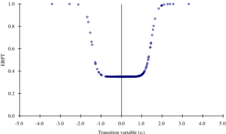
Based on the parameter estimates, we show the implied ERPT

f

^_2;0þ^

f

_4;0Gðzt; ^

g

ÞinFig. 4against

the transition variablezt ¼3 1P3j¼1

p

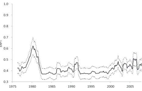
t j (the circles denoting the actual data points). The plot

suggests that the degree of ERPT becomes largest when the transition variable, namely the average lagged inflation rate, exceeds 2 percent in absolute value. Fig. 5 shows the smoothed estimates of the time-varying ERPT, based on the 12-month moving averages, along with their two-standard error bands. The smoothed plot illustrates three distinct high ERPT episodes. The

first high ERPT period corresponds to the second oil shock in the late 1970s. During the 1980s and 1990s, the ERPT is relatively stable except for the early 1990s when the producer price index is relatively volatile. During the decade beginning in 2000, the ERPT becomes high again due to the increased inflation.

4.3. Symmetric DLSTAR model

To select the delay parameter for the transition variable and lags for the regressors in a symmetric version of the DLSTAR model, we use a procedure similar to the one employed for the ESTAR model estimation. We selectd_¼1 and the estimation results are given as follows:

pt

¼0:098

ð3:466Þþ0:208ð3:866Þ

p

t 1þ0:159ð4:278Þ

p

t 3 0:101ð2:195Þ

p

t 5þð0:34912:519Þ

D

stþpt

þ0:075 ð2:341Þ

D

st 1þpt 1

_0:070 ð2:441Þ

D

st 2þpt 2

þ0:066 ð2:081Þ

D

st 5þpt 5

þh0:242

ð1:150Þ

p

t 4 0:739ð2:749Þ

p

t 5þ1:230ð5:269Þ

p

t 6þð0:65123:333Þ

D

stþpt

0:438 ð5:568Þ

D

st 1þpt 1

þ0:350 ð3:109Þ

D

st 2þpt 2

0:534 ð2:695Þ

D

st 4þpt 4

0:356 ð1:957Þ

D

st 5þpt 5 i

G_ðzt; ^

g

;^cÞ þ^3_t;

Fig. 5.ERPT over time: ESTAR model.

Gðzt;^

g

;^cÞ¼ 0

B B B @

1þexp

8 > > <

> > :

5:130 ð2:924Þ

p

t 1 1:474

ð21:283Þ

0:686 9 > > =

> > ; 1

C C C A 1

þ 0

B B B @

1þexp

8 > > <

> > :

5:130 ð2:924Þ 0

B B @

p

t 1þ1:474

ð21:283Þ 0:686

1

C C A 9 > > =

> > ; 1

C C C A 1

;

R2 ¼0:654;se ¼ 0:448;obs¼396;LMð1Þ ¼ 0:040;LMð1 12Þ ¼ 0:242:

Again, the estimate of the scaling parameter

g

(_¼

g

1¼

g

2) is expressed in terms of a normalized

transition variable. As shown inFig. 6, the shape of the implied ERPT

f

^2;0þ^

f

4;0Gðzt; ^

g

;^cÞas a function

of the transition variablezt ¼

p

t 1 somewhat resembles the shape of the transition function of TAR

model predicted by the two-period contract case (Fig. 1). A threshold-model-like shape of the tran-sition function results in many data points near the lowest ERPT. Because of this feature, the time series plot of ERPT based on the DLSTAR model shown inFig. 7shows more observations of low and stable ERPT around 0.35 compared to the case of the ESTAR model.

0.0 0.2 0.4 0.6 0.8 1.0

-5.0 -4.0 -3.0 -2.0 -1.0 0.0 1.0 2.0 3.0 4.0 5.0

Transition variable (z )

ERPT

Fig. 6.ERPT against the transition variable: symmetric DLSTAR model.

ER

P

T

Fig. 7. ERPT over time: symmetric DLSTAR model.

4.4. Asymmetric DLSTAR model

We now turn to the estimation of the asymmetric version of the DLSTAR model to incorporate the possibility of asymmetric adjustment. Minimizing the sum of the squared residuals yields the choice of d¼1. Thefinal specification of the model with parameter estimates is as follows:

pt

¼0:095

ð3:349Þþ0:270ð4:183Þ

p

t 1þ0:153ð4:094Þ

p

t 3 0:105ð2:326Þ

p

t 5þð0:34112:352Þ

D

stþpt

þ0:062 ð1:879Þ

D

st 1þpt 1

0:078 ð2:747Þ

D

st 2þpt 2

þ0:064 ð2:071Þ

D

st 5þpt 5

þh 0:198

ð1:722Þ

p

t 1 0:510ð1:979Þ

p

t 5þ1:001ð4:666Þ

p

t 6þð0:65923:868Þ

D

stþpt

0:338 ð3:324Þ

D

st 1þpt 1

þ0:417 ð3:352Þ

D

st 2þpt 2

0:298 ð2:685Þ

D

st 4þpt 4

0:482 ð2:699Þ

D

st 5þpt 5 i

G_ðzt; ^

g

1;

g

^2;^c1;^c2Þ þ^3_t;

G_ðzt; ^

g

1;^

g

2;^c1;^c2Þ ¼ 0

B B B @

1_þexp

8 > > < > > : 5:762 ð1:129Þ

p

_t 1 1:591

ð14:924Þ 0:686 9 > > = > > ; 1 C C C A 1 þ 0 B B B @

1þexp

8 > > < > > : 55:253 ð1:124Þ

p

t 1þ 1:293

ð156:218Þ 0:686 9 > > = > > ; 1 C C C A 1 ;

R2 _¼0:663;se _¼0:443;obs _¼396;LM_ð1_{Þ ¼} 0:073;LM_ð1 12_{Þ ¼}0:247:

Again, the estimates of the scaling parameters

g

1and

g

2are expressed in terms of the normalized

transition variable.

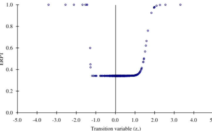
Fig. 8plots the implied ERPT

f

^_2;0þ

f

^_4;0Gðzt; ^

g

1;^

g

2;^c1;^c2Þagainst the transition variablezt ¼

p

t 1

allowing for the asymmetric adjustment. In terms of the shape of the transition function, the

0.0 0.2 0.4 0.6 0.8 1.0

-5.0 -4.0 -3.0 -2.0 -1.0 0.0 1.0 2.0 3.0 4.0 5.0

Transition variable (zt)

ERPT

Fig. 8.ERPT against the transition variable: asymmetric DLSTAR model.

asymmetric DLSTAR specification result is similar to that of the symmetric DLSTAR specification. However, because the estimate of

g

2is much larger than that of

g

1, the transition is much faster in the

negative region.Fig. 9shows the smoothed plots of the ERPT implied by the asymmetric DLSTAR model estimates over the sample period. The behavior of estimated ERPT is very similar to the one implied by the symmetric DLSTAR model.

4.5. Specification test

Table 2reports the results of the specification test to select an appropriate transition function among the ESTAR, the symmetric DLSTAR and the asymmetric DLSTAR models. In some cases, the null hypothesis of the ESTAR model against the asymmetric DLSTAR model cannot be rejected (seeF3with

dgreater than 3). On the other hand, the evidence suggests rejecting the symmetric DLSTAR model in favor of the asymmetric DLSTAR (F13) and the ESTAR specifications ðF1j3Þ. While the evidence is

somewhat mixed, the ESTAR and asymmetric DLSTAR speci_fications may be slightly better than the symmetric DLSTAR specification.

ER

P

T

Fig. 9.ERPT over time: asymmetric DLSTAR model.

Table 2

Specification tests for STAR models.

Test statistics Transition variableðzt¼d 1Pdj¼1ptejÞ

H0(H1) d¼1 d¼2 d¼3 d¼4 d¼5 d¼6

F3 ESTAR

(Asymmetric DLSTAR)

3.82 (0.00) 2.91 (0.00) 2.31 (0.01) 1.49 (0.13) 1.70 (0.06) 1.14 (0.32)

F1j3 Symmetric DLSTAR

(ESTAR)

2.70 (0.00) 3.00 (0.00) 2.74 (0.00) 2.97 (0.00) 2.28 (0.01) 1.27 (0.23)

F13 Symmetric DLSTAR

(Asymmetric DLSTAR)

3.04 (0.00) 2.76 (0.00) 2.37 (0.00) 2.10 (0.07) 1.89 (0.02) 1.16 (0.29)

Lag length isN¼6.F3is the F test statistic forH0:b3¼0 againstH1:b3s_0.F1

j3is the F test statistic forH0:b1 ¼0jb3¼0 againstH1:b1s0jb3 ¼0.F13is the F test statistic forH0:b1 ¼b3 ¼0 againstH1:b1s0 andb3s0. Under the null hypothesis, three sets of F test statistics follow F distributions withð2N;T 8N 1Þ,ð2N;T 6N 1Þandð4N;T 8N 1Þdegrees of freedom, respectively. The numbers in parentheses below F statistics arep-values.

5. Conclusion

In this paper, we show that the STAR models, the parsimonious parametric nonlinear time series models, offer a very convenient framework in examining the relationship between the ERPT and inflation. First, a simple theoretical model of ERPT determination suggests that the dynamics of ERPT can be well approximated by a class of STAR models with lagged in_flation as a transition variable. Second, we can employ various U-shaped transition functions in the estimation of the time-varying ERPT. When this procedure is applied to US import and domestic price data, wefind the supporting evidence of nonlinearity in ERPT dynamics. Our empirical results imply that the period of low ERPT is likely to be associated with the low inflation.

According to our model, the degree of ERPT varies over time because the fraction of importingfirms opting out from the contract is endogenously determined by importingfirms’optimization behavior. In the model, however, all imports are treated as if they are invoiced in the producer’s (exporter’s) currency. An alternative approach in introducing a time-varying ERPT is to use a model in which exportingfirms endogenously choose between producer currency pricing (PCP) and local currency pricing (LCP). For example, a recent study byGopinath et al. (2010)extends the model ofEngel (2006)

and investigates the role of the invoice currency in determining the observed ERPT. Our analysis does not consider this channel partly because we do not have data on individual exporters’invoice currency. Incorporating the effect of currency choice in our estimation procedure seems to be a promising direction for further analysis.

Acknowledgment

The authors gratefully acknowledge an anonymous referee, the Editor, Mick Devereux, Ippei Fuji-wara, Naohisa Hirakata, Kevin Huang, Nobu Kiyotaki, Takushi Kurozumi, Keisuke Otsu, Shigenori Shiratsuka and seminar and conference participants at the Georgia Institute of Technology, Osaka University, the University of Texas at Arlington and the 2009 Far East and South Asia Meeting of the Econometric Society for their helpful comments and discussions. Shintani gratefully acknowledges

financial support by the National Science Foundation Grant SES-1030164. The views expressed in the paper are those of the authors and are not re_flective of those of the Asian Development Bank.

Appendix: Model of importers

In this appendix we provide a full description of the theoretical model and derive its implications discussed in Section2. There is a continuum of monopolistically competitive importingfirms, each of which imports a differentiated intermediate good from abroad and sells it to a representative domestic

final good producer. In each time period, a constant fraction 1 /Nof all importingfirms and thefinal good producer write their pricing contracts ofNperiods long. An importingfirm that writes the pricing contract at timete_{j(forj ¼0;1;}._{;N 1) and imports a goodi}˛_{½0;1Š, at timetis facing a demand}

given by

Ctði;t jÞ ¼ _P

tði;t jÞ

Ptðt jÞ

q

Ctðt jÞ

where

q

>1 is a constant elasticity of substitution. Here, Ptði;t jÞ is the price of a good i

imported by afirm with a contract beginning in periodt j.Ptðt jÞ ¼ ðR01Ptði;t jÞ1 qdiÞ1=ð1 qÞis

the price index for the composite intermediate good sold by importing _firms whose contracts begin in periodt j.Ctðt jÞis the demand for the corresponding composite good. The elasticity

of substitution among composite intermediate goods sold by each fraction 1/Nof all importing

firms is assumed to be one, and thus aggregate price index at time t (in log) is pt ¼ N 1PNj¼01ptðt jÞ whereptðt jÞ ¼lnPtðt jÞ.

All the differentiated intermediate goods are imported at the same foreign currency price,P t, which

is beyond the control of importers. The importer’s pro_fit, in terms of the domestic currency, at timetis given by

P

tði;t jÞ ¼Ptði;t jÞCtði;t jÞ ð1þ

s

ÞS_tP

tCtði;t jÞ

whereStis the nominal exchange rate, and

s

is the iceberg transportation cost the importer must bear. The importer’s desired price, which maximizes the profit underflexible price economy, is

^

Ptði;t jÞ ¼

q

q

1ð1þ

s

ÞStPt

where

q

=ð

q

1_Þ, and_ð1_þ

s

_ÞS_tP

t represent the mark-up and marginal cost, respectively. By taking a log

of the desired price, which is same across all the importingfirms_ð^Pt ¼^Ptði;t jÞÞ, we havep^t ¼stþ p

tþ

m

where st ¼lnSt and

m

¼lnð

q

=ð

q

1ÞÞ þlnð1þ

s

Þ. Both s_t and p

t are assumed to follow

(possibly mutually correlated) random walk processes with a variance of the sum of each increment,

D

_ðstþptÞ, given by

s

2.

In the initial period of the contract, importers set the price at^pt. For the rest of the contract

period, they fully index their initial price^p_tto the aggregate inflation rate given by

p

t ¼ pt pt 1.

Note that prices are indexed to inflation of the initial period only, instead of following the period-by-period lagged inflation indexation rule as in Christiano et al. (2005). While the latter pricing scheme can be also introduced in our model, the former assumption greatly simpli_fies the analysis.

In reality, contracts written forfixed periods can, in special circumstances, be re-negotiated. By paying afixed cost,firms can opt out of the contract and reset their price at the desired level. For example, inDevereux and Siu (2007), eachfirm observes its fix cost, which is assumed to be i.i.d. acrossfirms, after setting its (two-period) contract price. Consequently, the pricing in the second period becomes state-dependent with all firms facing the same probability of opting out in the second period. We also letfirms make their decision in a sequential manner by assuming that the aggregate inflation is not observed by individualfirms at the time of the contract. However, instead of formally deriving the state-dependent pricing solution, we followBall et al. (1988), Romer (1990), and

Devereux and Yetman (2002, 2010), among others, and re-formulate thefirm’s optimization behavior so that the probability of (not) changing its price to the desired price level is endogenously deter-mined. Let

k

ðtÞ_{be the conditional probability that afirm will not opt out of the contract, provided that} the_firm is in the contract in the current period. After setting the new contract price^ptatt, thefirms

observe the aggregate inflation

p

tand choose

k

ðtÞto maximize their profit. As inWalsh (2003), we can

rewrite the intertemporal profit maximization condition using the expected squared deviation of the actual price from the desired price in each period.

(A) Two-period contract case

WhenN_¼2, an optimal value of

k

ðtÞ_{is selected by minimizing the expected loss function given by}

Lt ¼Et h

bk

ðtÞ_ð^p_tþ

p

t p^tþ1Þ2 i

þ

b

1

k

ðtÞ

F

¼

b

F

b

F

s

2

_p

2

t

k

ðtÞ

where

b

is a discount factor andFis afixed cost. Here we exclude the possibility ofF<

s

2_{, since}

the loss is always minimized by setting

k

ðtÞ _{¼0 in such a case. WhenF}

_s

2_{, thefirm selects}

_k

ðtÞ _{¼1 if}

p

2

t F

s

2and

k

ðtÞ ¼0 if

p

2t >F

s

2. Thus, for the given values ofFand

s

2,

k

ðtÞis simply a function of

p

t. When we use the same argument, for anyfirms entering into contracts at timet ej,

k

ðt jÞ is

a function of

p

_{t j}given by

k

_ð

p

_{t jÞ ¼}1fj

p

_{t jj} ffiffiffiffiffiffiffiffiffiffiffiffiffiffi

F

s

2

p

g. Using the definition of the aggregate price index, we have

pt ¼ 1

2ðptðtÞ þptðt 1ÞÞ ¼

stþpt þ

m

k

ð

p

t 1Þ

2

D

stþpt

since thefirms with new contracts set their priceptðtÞat the desired price,p^t ¼stþptþ

m

, and the

firms with contracts made in the previous period set their price ptðt 1Þ at ð1

k

_ð

p

t 1ÞÞ^ptþ

k

ð

p

t 1Þð^pt 1þ

p

t 1Þ. The inflation dynamics are written as

p

t ¼

1

k

ð

p

t 1Þ 2

D

stþpt

þ

k

ð

p

₂t 2Þ

D

s_t 1þpt 1

þ

k

ð

p

₂t 1Þ

p

_t 1

k

_ð

p

_{t 2Þ} 2

p

t 2:

We followDevereux and Yetman (2010), among others, and consider the (short-run) ERPT in terms of thefirst derivative of

p

twith respect to

D

ðstþptÞ, or

ERPT ¼1

k

ð

p

t 1Þ 2 ;

which depends on the lagged inflation,

p

t 1. When

ffiffiffiffiffiffiffiffiffiffiffiffiffiffi

F

s

2

p

p

t 1

ffiffiffiffiffiffiffiffiffiffiffiffiffiffi

F

s

2

p

,

k

_ð

p

t 1Þtakes a value of

one and the ERPT becomes 0.5. On the other hand, whenj

p

t 1j> ffiffiffiffiffiffiffiffiffiffiffiffiffiffi

F

s

2

p

, the model predicts a full ERPT.

(B) Three-period contract case

WhenN¼3, the loss function becomes a quadratic function of

k

ðtÞ_{given by}

Lt¼Et h

bk

ðtÞ_ð^p_tþ

p

t p^tþ1Þ2þ

bk

ðtÞ2_ð^p_tþ2

p

t ^ptþ2Þ2 i

þ

b

1

k

ðtÞ_ð1þ

_b

_ÞFþ

_b

2

_k

_ðtÞ₁

_k

ðtÞ_F

¼

b

_ð1_þ

b

_ÞF

b

F

s

2

_p

2 t

k

ðtÞ

_b

2

F 2

s

2 ₄

_p

2 t

k

ðtÞ2

:

Thefirst-order condition yields the optimal

k

ðtÞ_{given by}

k

_ð

pt

_{Þ ¼}

F

s

2

_p

2

t

2

b

F 2

s

2 ₄

_p

2 t

provided F

s

2

_p

2

t >0 and ðF

s

2

p

2tÞ þ2

b

ðF 2

s

2 4

p

2tÞ<0. In this case,

k

ðtÞ is a smooth

function of the inflation rate

p

t. Otherwise,

k

ðtÞbecomes a corner solution taking a value of either0or1.

In particular, if F

s

2

_p

2

t >0 and ðF

s

2

p

2tÞ þ2

b

ðF 2

s

2 4

p

2tÞ 0, then

k

ð

p

tÞ ¼1. If

F

s

2

_p

2

t 0, then

k

ð

p

tÞ ¼0. The aggregate price is given by

pt¼1₃ðptðtÞþptðt 1Þþptðt 2ÞÞ

¼

stþpt

k

ð

p

t 1Þþ

k

ð

p

t 2Þ2

3

D

stþpt

k

ð

p

t 2Þ2

3

D

st 1þpt 1

þ

k

ð

p

₃t 1Þ

p

_t 1þ2

k

ð

p

t 2Þ 2

3

p

t 2

where the second equality follows from ptðt 1Þ ¼ ð1

k

ð

p

t 1ÞÞ^ptþ

k

ð

p

t 1Þðp^t 1þ

p

t 1Þ and

ptðt 2Þ ¼ ð1

k

ð

p

t 2Þ2Þ^ptþ

k

ð

p

t 2Þ2ð^pt 2þ2

p

t 2Þ. The inflation dynamics are given by

p

t ¼ 1

k

ð

p

t 1Þ þ

k

ð

p

t 2Þ 2

3

!

D

_s tþpt

1 3

k

_ð

p

_t 2Þ2

k

ð

p

t 2Þ

k

ð

p

t 3Þ2

D

_s

t 1þpt 1

þ

k

ð

p

t 3Þ 2

3

D

st 2þpt 2

þ

k

ð

p

₃t 1Þ

p

t 1þ

1 3

2

k

ð

p

t 2Þ2

k

ð

p

t 2Þ

p

t 2

2

k

_ð

p

_t 3Þ2

3

p

t 3:

The ERPT is given by

ERPT _¼1

k

ð

p

t 1Þ þ

k

ð

p

t 2Þ

2

3

which now depends on

p

t 1and

p

t 2.

(C) N-period contract case

Using a similar argument, for general N, the current inflation becomes a function of

p

_{t j} for j _¼1;._;Nand

D

_ðs_{t jþ}p

t jÞforj ¼0;.;N 1. The ERPT for anyNis given by

ERPT ¼1

PN 1

j¼1

k

p

t jj

N

where

k

_ð

p

t jÞis a nonlinear function of

p

t j. The second termN 1PNj¼11

k

ð

p

t jÞjrepresents the fraction

offirms adapting the indexation rule and the ERPT can now vary from 1/Nto1. In general, the ERPT is a smooth nonlinear function of lagged in_flation rates, with its dynamics possibly approximated by STAR models with a U-shaped transition function.

References

Ball, L., Mankiw, N.G., 1994. Asymmetric price adjustment and economicfluctuations. Economic Journal 104, 247e261. Ball, L., Mankiw, N.G., Romer, D., 1988. The new Keynesian economics and the output-inflation trade-off. Brookings Papers on

Economic Activity 1, 1e65.

Bec, F., Ben Salem, M., Carrasco, M., 2004. Detecting mean reversion in real exchange rates from a multiple regime STAR model. Mimeo. Calvo, G.A., Reinhart, C.M., 2002. Fear offloating. Quarterly Journal of Economics 117 (2), 379e408.

Campa, J.M., Goldberg, L.S., 2005. Exchange rate pass-through to domestic prices. Review of Economics and Statistics 87 (4), 679e690. Choudhri, E.U., Hakura, D.S., 2006. Exchange rate pass-through to domestic prices: does the inflationary environment matter?

Journal of International Money and Finance 25 (4), 614e639.

Choudhri, E.U., Faruqee, H., Hakura, D.S., 2005. Explaining the exchange rate pass-through in different prices. Journal of International Economics 65 (2), 349e374.

Christiano, L.J., Eichenbaum, M., Evans, C.L., 2005. Nominal rigidities and the dynamic effects of a shock to monetary policy. Journal of Political Economy 113, 1e45.

Devereux, M.B., Siu, H.E., 2007. State dependent pricing and business cycle asymmetries. International Economic Review 48 (1), 281e310.

Devereux, M.B., Yetman, J., 2002. Menu costs and the long-run output-inflation trade-off. Economics Letters 76, 95e100. Devereux, M.B., Yetman, J., 2010. Price adjustment and exchange pass-through. Journal of International Money and Finance 29,

181e200.

Engel, C., 2006. Equivalence results for optimal pass-through, optimal indexing to exchange rates, and optimal choice of currency for export pricing. Journal of the European Economic Association 4 (6), 1249e1260.

Goldberg, P.K., Knetter, M.M., 1997. Goods prices and exchange rates: what have we learned? Journal of Economic Literature 35, 1243e1272.

Gopinath, G., Itskhoki, O., Rigobon, R., 2010. Currency choice and exchange rate pass-through. American Economic Review 100 (1), 304e336.

Granger, C.W.J., Teräsvirta, T., 1993. Modelling Nonlinear Economic Relationships. Oxford University Press, Oxford.

Haggan, V., Ozaki, T., 1981. Modelling nonlinear random vibrations using an amplitude-dependent autoregressive time series model. Biometrika 68 (2), 189e196.

Herzberg, V., Kapetanios, G., Price, S., 2003. Import prices and exchange rate pass-through: Theory and evidence from the United Kingdom. Bank of England Working Paper, No. 182.

Kilian, L., Taylor, M.P., 2003. Why is it so difficult to beat the random walk forecast of exchange rates? Journal of International Economics 60, 85e107.

McCarthy, J., 2007. Pass-through of exchange rates and import prices to domestic inflation in some industrialized economies. Eastern Economic Journal 33 (4), 511e537.

Michael, P., Nobay, A.R., Peel, D.A., 1997. Transaction costs and nonlinear adjustments in real exchange rates: an empirical investigation. Journal of Political Economy 105, 862e879.

Otani, A., Shiratsuka, S., Shirota, T., 2003. The decline in the exchange rate pass-through: evidence from Japanese import prices. Bank of Japan Monetary and Economic Studies 21 (3), 53e81.

Romer, D., 1990. Staggered price setting with endogenous frequency of adjustment. Economics Letters 32, 205e210. Sekine, T., 2006. Time-varying exchange rate pass-through: Experiences of some industrial countries. BIS Working Paper, No. 202. Taylor, J.B., 1980. Aggregate dynamics and staggered contracts. Journal of Political Economy 88, 1e23.

Taylor, J.B., 2000. Low inflation, pass-through, and the pricing power offirms. European Economic Review 44, 1389e1408. Taylor, M.P., Peel, D.A., 2000. Nonlinear adjustment, long-run equilibrium and exchange rate fundamentals. Journal of

Inter-national Money and Finance 19, 33e53.

Taylor, M.P., Peel, D.A., Sarno, L., 2001. Nonlinear mean-reversion in real exchange rates: toward a solution to the purchasing power parity puzzles. International Economic Review 42, 1015e1042.

Teräsvirta, T., 1994. Specification, estimation, and evaluation of smooth transition autoregressive models. Journal of the American Statistical Association 89, 208e218.

van Dijk, D., Teräsvirta, T., Franses, P., 2002. Smooth transition autoregressive models: a survey of recent developments. Econometrics Reviews 21, 1e47.

Walsh, C.E., 2003. Monetary Theory and Policy, second ed. MIT Press, Cambridge.