鹿児島大学リポジトリ

(1)

Linear Discrete-Time Stochastic Systems

著者

NAKAMORI Seiichi

journal or

publication title

Bulletin of the Faculty of Education,

Kagoshima University. Natural science

volume

66 page range

51-66

(2)

Design of RLS Wiener Fixed-Lag Smoother in Linear Discrete-Time

Stochastic Systems

NAKAMORI Seiichi (Received , 2014)

Abstract

This paper newly presents the recursive least-squares (RLS) fixed-lag smoother using the covariance information and then the RLS Wiener fixed-lag smoother in linear discrete-time wide-sense stationary stochastic systems. Here, the additional disturbance in the measurement of the signal is white noise. The signal is uncorrelated with observed noise. It is assumed that the signal process is fitted to the autoregressive (AR) model of order 𝑁𝑁. For this AR model of order 𝑁𝑁, in the proposed fixed-lag smoother, the fixed-lag smoothing estimate for the fixed lag 𝐿𝐿, 1 ≤ 𝐿𝐿 ≤ 𝑁𝑁 − 1, can be calculated. The RLS Wiener fixed-lag smoother requires information of the system matrix, the autovariance function of the state vector, the observation vector, the variance of the observation noise and the coefficients for 𝐾𝐾(𝑘𝑘 − 𝐿𝐿, 𝑠𝑠) in (19). It is advantageous that the proposed RLS Wiener fixed-lag smoother shows stable and feasible estimation characteristics in comparison with the RLS Wiener fixed-lag smoother [9].

Keyword：Discrete-time stochastic systems, RLS Wiener fixed-lag smoother, covariance information, Wiener-Hopf equation

___________________________

*_{Professor of Kagoshima University, Faculty of Education}

Design of RLS Wiener Fixed-Lag Smoother in Linear Discrete-Time

Sto-chastic Systems

N

AKAMORI

S

eiichi* (Received 28 October, 2014)

Abstract

(3)

1. Introduction

In control and communication systems, within acceptable delay, the smoothing estimate with improved estimation accuracy is preferable to the filtering estimate [1]. Also, it is pointed out that some fixed-lag smoothing algorithms in the literature, for example [2], [3], [4], are computationally unstable and therefore impractical. In the fixed-lag smoother the estimate 𝑧𝑧̂(𝑘𝑘 − 𝐿𝐿, 𝑘𝑘), at time 𝑘𝑘 − 𝐿𝐿, of the signal 𝑧𝑧(𝑘𝑘 − 𝐿𝐿) uses measurements until 𝑘𝑘. The fixed-lag smoothing algorithm developed in [1] utilizes the augmented state equation. In this method, the Kalman filter [5] is applicable to the augmented state equation for recursive calculation of the linear least-squares fixed-lag smoothing estimates. Moore [1] proposes various stable fixed-lag smothers for the finite-dimensional state-space model.

From the previous works in the literature, the fixed-point smoother with the following viewpoints might be useful. (1) In contrast to the filter, the fixed-lag smoother with improved estimation accuracy is advantageous. (2) Contrary to the unstable smoothers, computationally stable fixed-lag smoother is indispensable.

In [6], Nakamori et al., using the covariance information, propose the recursive least-squares (RLS) fixed-lag smoother. However, from the restriction that the covariance function of the signal is expressed in the degenerate kernel form, the smoother is not suitable for estimating the general stochastic signal processes with the autocovariance function in the semi-degenerate kernel form.

Previously, in linear discrete-time stochastic systems, the RLS Wiener fixed-point smoother [7], the RLS Wiener fixed-lag smoother [8], [9] and the RLS fixed-lag smoother [9], [10] using the covariance information are proposed. Also, the RLS fixed-lag smoother [11] using the covariance information is presented in linear continuous-time stochastic systems.

To avoid the undesirable instability of the RLS Wiener fixed-lag smoother, the aim of this paper is to design the computationally stable RLS Wiener fixed-lag smoother for the signal observed with additive white noise. The signal is uncorrelated with the observation noise. It is assumed that the signal process is fitted to the autoregressive (AR) model of order 𝑁𝑁. The key idea adopted in this paper is to express the autocovariance function 𝐾𝐾(𝑘𝑘 − 𝐿𝐿, 𝑠𝑠) of the signal, which appears in (8), by (19) for the fixed lag 𝐿𝐿, 1 ≤ 𝐿𝐿 ≤ 𝑁𝑁 − 1. Since 𝐾𝐾(𝑘𝑘 − 𝐿𝐿, 𝑠𝑠) is expressed as a linear combination of 𝐾𝐾(𝑘𝑘, 𝑠𝑠), 𝐾𝐾(𝑘𝑘 + 1, 𝑠𝑠), ⋯, 𝐾𝐾(𝑘𝑘 + 𝐿𝐿, 𝑠𝑠), 1 ≤ 𝑠𝑠 ≤ 𝑘𝑘 (see (19)), the invariant imbedding method used in the derivation of the RLS Wiener estimators [7] can be applied to the derivations of the current fixed-lag smoothing algorithms. As a step for obtaining the RLS Wiener fixed-lag smoothing algorithm in Theorem 2, the fixed-lag smoothing algorithm using the covariance information is proposed in Theorem 1. Here, it should be noted that the instability of the fixed-lag smoother in Theorem 1 might be caused by Φ−𝑘𝑘_{, included in 𝐵𝐵}𝑇𝑇_{(𝑘𝑘), for large}

(4)

Wiener fixed-lag smoother requires the information of the system matrix Φ, the autovariance function 𝐾𝐾𝑥𝑥(𝑘𝑘, 𝑘𝑘) of the state vector 𝑥𝑥(𝑘𝑘) , the observation vector 𝐻𝐻 and the coefficients 𝑎𝑎̄𝑖𝑖,𝑁𝑁 ,

𝑖𝑖 = 1, 2, ⋯ , 𝐿𝐿 + 1, in (19).

In section 5, by introducing the fixed-lag smoothing error variance function, it is shown that the current RLS Wiener fixed-lag smoother is stable.

In section 6, two numerical simulation examples are demonstrated to show the stable and feasible estimation characteristics of the current RLS Wiener fixed-lag smoother. From the viewpoints of the estimation accuracy and the stability, the proposed RLS Wiener fixed-lag smoother is superior to the RLS Wiener fixed-lag smoother [9]. In the numerical simulation examples, the signal processes are fitted to the AR model of order 𝑁𝑁 = 10.

2. Linear least-squares fixed-lag smoothing problem

Let a scalar observation equation and a state-space model be given by 𝑦𝑦(𝑘𝑘) = 𝑧𝑧(𝑘𝑘) + 𝑣𝑣(𝑘𝑘), 𝑧𝑧(𝑘𝑘) = 𝐻𝐻𝑥𝑥(𝑘𝑘),

𝑥𝑥(𝑘𝑘 + 1) = Φ𝑥𝑥(𝑘𝑘) + Γ𝑤𝑤(𝑘𝑘), (1)

in linear discrete-time wide-sense stationary stochastic systems. Here, 𝑧𝑧(𝑘𝑘) is signal, 𝐻𝐻 is the 1 × 𝑁𝑁 observation vector, 𝑥𝑥(𝑘𝑘) is the state vector, 𝑣𝑣(𝑘𝑘) is white observation noise, Φ is the system matrix and 𝑤𝑤(𝑘𝑘) is the white noise input, which is uncorrelated with the observation noise. It is also assumed that the signal and the observation noise are zero mean and mutually independent. Let the autocovariance function of 𝑣𝑣(𝑘𝑘) be given by

𝐸𝐸[𝑣𝑣(𝑘𝑘)𝑣𝑣𝑇𝑇_{(𝑠𝑠)] = 𝑅𝑅𝛿𝛿}

𝐾𝐾(𝑘𝑘 − 𝑠𝑠), 𝑅𝑅 > 0. (2)

Here, 𝛿𝛿𝐾𝐾(⋅) denotes the Kronecker 𝛿𝛿 function.

Let 𝐾𝐾(𝑘𝑘, 𝑠𝑠) represent the autocovariance function of 𝑧𝑧(𝑘𝑘) and let 𝐾𝐾(𝑘𝑘, 𝑠𝑠) be expressed in the semi-degenerate kernel form of

𝐾𝐾(𝑘𝑘, 𝑠𝑠) = �𝐴𝐴(𝑘𝑘)𝐵𝐵_{𝐵𝐵(𝑘𝑘)𝐴𝐴}𝑇𝑇_𝑇𝑇(𝑠𝑠), 0 ≤ 𝑠𝑠 ≤ 𝑘𝑘,_{(𝑠𝑠), 0 ≤ 𝑘𝑘 ≤ 𝑠𝑠.} (3) Hypothesis of (3) is motivated by the fact that in many applications the covariance function of the signal to be estimated admits a semi-degenerate kernel form. Note that when the system matrix Φ in the state-space model, the observation vector 𝐻𝐻 in the observation equation and the variance 𝐾𝐾𝑥𝑥(𝑘𝑘, 𝑘𝑘) of the state vector

are available, the signal autocovariance function can be expressed as 𝐾𝐾(𝑘𝑘, 𝑠𝑠) = 𝐻𝐻Φ𝑘𝑘−𝑠𝑠_𝐾𝐾

𝑥𝑥(𝑠𝑠, 𝑠𝑠)𝐻𝐻𝑇𝑇, 𝑠𝑠 ≤ 𝑘𝑘,

(5)

Φ−𝑠𝑠_𝐾𝐾

𝑥𝑥(𝑠𝑠, 𝑠𝑠)𝐻𝐻𝑇𝑇[9] and clearly, this factorization is not unique. Actually, processes with finite-dimensional

state-space models, have covariance functions expressed in the semi-degenerate kernel form (3). Consequently, since this semi-degenerate kernel form is suitable for expressing autocovariance functions of stochastic signals in general, the fixed-lag smoothing algorithm proposed in the paper have a wide applicability.

Let a fixed-lag smoothing estimate 𝑧𝑧̂(𝑘𝑘 − 𝐿𝐿, 𝑘𝑘) of 𝑧𝑧(𝑘𝑘 − 𝐿𝐿) be given by 𝑧𝑧̂(𝑘𝑘 − 𝐿𝐿, 𝑘𝑘) = � ℎ

𝑘𝑘 𝑖𝑖=1

(𝑘𝑘, 𝑖𝑖)𝑦𝑦(𝑖𝑖) (4)

as a linear transformation of the observed values {𝑦𝑦(𝑖𝑖), 1 ≤ 𝑖𝑖 ≤ 𝑘𝑘}. Here, ℎ(𝑘𝑘, 𝑖𝑖) and 𝐿𝐿 are called the impulse response function and the fixed lag.

The impulse response function, which minimizes the mean-square value of the fixed-lag smoothing error 𝑧𝑧(𝑘𝑘 − 𝐿𝐿) − 𝑧𝑧̂(𝑘𝑘 − 𝐿𝐿, 𝑘𝑘),

𝐽𝐽 = 𝐸𝐸[‖𝑧𝑧(𝑘𝑘 − 𝐿𝐿) − 𝑧𝑧̂(𝑘𝑘 − 𝐿𝐿, 𝑘𝑘)‖2_], ₍₅₎

satisfies that the estimation error 𝑧𝑧(𝑘𝑘 − 𝐿𝐿) − 𝑧𝑧̂(𝑘𝑘 − 𝐿𝐿, 𝑘𝑘) is orthogonal to the observations [2]; that is 𝐸𝐸[(𝑧𝑧(𝑘𝑘 − 𝐿𝐿) − 𝑧𝑧̂(𝑘𝑘 − 𝐿𝐿, 𝑘𝑘))𝑦𝑦𝑇𝑇_{(𝑠𝑠)] = 0, 1 ≤ 𝑠𝑠 ≤ 𝑘𝑘.} ₍₆₎

From (4) and (6), the Wiener-Hopf equation, which the impulse response satisfies, is given by 𝐾𝐾(𝑘𝑘 − 𝐿𝐿, 𝑠𝑠) = � ℎ

𝑘𝑘 𝑖𝑖=1

(𝑘𝑘, 𝑖𝑖)𝐸𝐸[𝑦𝑦(𝑖𝑖)𝑦𝑦𝑇𝑇_(𝑠𝑠)]. ₍₇₎

Substituting (1) into (7) and using (2), we obtain ℎ(𝑘𝑘, 𝑠𝑠)𝑅𝑅 = 𝐾𝐾(𝑘𝑘 − 𝐿𝐿, 𝑠𝑠) − � ℎ

𝑘𝑘 𝑖𝑖=1

(𝑘𝑘, 𝑖𝑖)𝐾𝐾(𝑖𝑖, 𝑠𝑠). (8)

(8) is the basic equations, which the impulse response function ℎ(𝑘𝑘, 𝑠𝑠) satisfies, for deriving the RLS fixed-lag smoothing algorithm using the covariance information and the RLS Wiener fixed-lag smoothing algorithm of the signal in linear discrete-time stochastic systems.

3. AR model for the signal process

Let us assume that the signal process is fitted to the AR model of order 𝑁𝑁.

𝑧𝑧(𝑘𝑘) = −𝑎𝑎1𝑧𝑧(𝑘𝑘 − 1) − 𝑎𝑎2𝑧𝑧(𝑘𝑘 − 2) − ⋯ − 𝑎𝑎𝑁𝑁𝑧𝑧(𝑘𝑘 − 𝑁𝑁) + 𝑤𝑤(𝑘𝑘). (9)

It is seen that the 1 × 𝑁𝑁 observation vector 𝐻𝐻 in (1) and the state equation for the state vector 𝑥𝑥(𝑘𝑘) are expressed as follows:

(6)

𝐻𝐻 = [1 0 0 ⋯ 0], (10) ⎣ ⎢ ⎢ ⎢ ⎡ 𝑥𝑥_𝑥𝑥1(𝑘𝑘 + 1) 2(𝑘𝑘 + 1) ⋮ 𝑥𝑥𝑁𝑁−1(𝑘𝑘 + 1) 𝑥𝑥𝑁𝑁(𝑘𝑘 + 1) ⎦ ⎥ ⎥ ⎥ ⎤ = ⎣ ⎢ ⎢ ⎢ ⎡ 0₀ 1₀ 0₁ _⋯⋯ 0₀ 0₀ ⋮ ⋮ ⋮ ⋱ ⋮ ⋮ 0 0 0 ⋯ 0 1 −𝑎𝑎𝑁𝑁 −𝑎𝑎𝑁𝑁−1 −𝑎𝑎𝑁𝑁−2 ⋯ −𝑎𝑎2 −𝑎𝑎1⎦ ⎥ ⎥ ⎥ ⎤ ⎣ ⎢ ⎢ ⎢ ⎡ 𝑥𝑥_𝑥𝑥1(𝑘𝑘) 2(𝑘𝑘) ⋮ 𝑥𝑥𝑁𝑁−1(𝑘𝑘) 𝑥𝑥𝑁𝑁(𝑘𝑘) ⎦ ⎥ ⎥ ⎥ ⎤ + ⎣ ⎢ ⎢ ⎢ ⎡0₀ ⋮ 0 1⎦⎥ ⎥ ⎥ ⎤ 𝑤𝑤(𝑘𝑘), (11) 𝐸𝐸[𝑤𝑤(𝑘𝑘)𝑤𝑤(𝑠𝑠)] = 𝑄𝑄𝛿𝛿𝐾𝐾(𝑘𝑘 − 𝑠𝑠). ₍₁₂₎

In (8), the autocovariance function 𝐾𝐾(𝑘𝑘 − 𝐿𝐿, 𝑠𝑠), 1 ≤ 𝑘𝑘 − 𝐿𝐿, 𝑠𝑠 ≤ 𝑘𝑘, 𝐿𝐿 = 1, 2, ⋯ , 𝑁𝑁 − 2, 𝑁𝑁 − 1, can not be expressed in the form (3) of the semi-degenerate kernel.

In (9), by proceeding the time 𝑘𝑘 by 𝑁𝑁 − 1, the following equation is obtained.

𝑧𝑧(𝑘𝑘 + 𝑁𝑁 − 1) = −𝑎𝑎1𝑧𝑧(𝑘𝑘 + 𝑁𝑁 − 2) − 𝑎𝑎2𝑧𝑧(𝑘𝑘 + 𝑁𝑁 − 3) − ⋯ − 𝑎𝑎𝑁𝑁𝑧𝑧(𝑘𝑘 − 1) + 𝑤𝑤(𝑘𝑘 + 𝑁𝑁 − 1). (13)

By postmultiplying 𝑧𝑧(𝑠𝑠) to (13) and taking into considerations of the relationship 𝐾𝐾(𝑘𝑘, 𝑠𝑠) = 𝐸𝐸[𝑧𝑧(𝑘𝑘)𝑧𝑧(𝑠𝑠)], 𝐾𝐾(𝑘𝑘 + 𝑁𝑁 − 1, 𝑠𝑠)

= −𝑎𝑎1𝐾𝐾(𝑘𝑘 + 𝑁𝑁 − 2, 𝑠𝑠) − 𝑎𝑎2𝐾𝐾(𝑘𝑘 + 𝑁𝑁 − 3, 𝑠𝑠) − ⋯ − 𝑎𝑎𝑁𝑁𝐾𝐾(𝑘𝑘 − 1, 𝑠𝑠)

(14) is valid. From (14), we see that

𝐾𝐾(𝑘𝑘 − 1, 𝑠𝑠) = (𝐾𝐾(𝑘𝑘 + 𝑁𝑁 − 1, 𝑠𝑠) + 𝑎𝑎1𝐾𝐾(𝑘𝑘 + 𝑁𝑁 − 2, 𝑠𝑠) + 𝑎𝑎2𝐾𝐾(𝑘𝑘 + 𝑁𝑁 − 3, 𝑠𝑠)

+ ⋯ + 𝑎𝑎𝑁𝑁−1𝐾𝐾(𝑘𝑘, 𝑠𝑠))/(−𝑎𝑎𝑁𝑁). (15)

Similarly, the equations (16)-(18) are obtained.

+ ⋯ + 𝑎𝑎𝑁𝑁−1𝐾𝐾(𝑘𝑘 − 1, 𝑠𝑠))/(−𝑎𝑎𝑁𝑁) (16)

(7)

⋅⋅⋅⋅⋅⋅⋅⋅⋅⋅⋅⋅⋅⋅⋅⋅⋅⋅⋅⋅⋅⋅⋅⋅⋅⋅⋅⋅⋅⋅⋅⋅⋅⋅⋅⋅⋅⋅

𝐾𝐾(𝑘𝑘 − (𝑁𝑁 − 1), 𝑠𝑠) = (𝐾𝐾(𝑘𝑘 + 1, 𝑠𝑠) + 𝑎𝑎1𝐾𝐾(𝑘𝑘, 𝑠𝑠) + 𝑎𝑎2𝐾𝐾(𝑘𝑘 − 1, 𝑠𝑠)

+ ⋯ + 𝑎𝑎𝑁𝑁−1𝐾𝐾(𝑘𝑘 − (𝑁𝑁 − 2), 𝑠𝑠))/(−𝑎𝑎𝑁𝑁) (18)

𝐾𝐾(𝑘𝑘 − 1, 𝑠𝑠) is given by (15) in terms of 𝐾𝐾(𝑘𝑘 + 𝑖𝑖 − 1, 𝑠𝑠), 1 ≤ 𝑖𝑖 ≤ 𝑁𝑁. By substituting (15) into (16), 𝐾𝐾(𝑘𝑘 − 2, 𝑠𝑠) is expressed in terms of 𝐾𝐾(𝑘𝑘 + 𝑖𝑖 − 1, 𝑠𝑠), 1 ≤ 𝑖𝑖 ≤ 𝑁𝑁. By successive substitutions, 𝐾𝐾(𝑘𝑘 − (𝑁𝑁 − 1), 𝑠𝑠) is also expressed in terms of 𝐾𝐾(𝑘𝑘 + 𝑖𝑖 − 1, 𝑠𝑠), 1 ≤ 𝑖𝑖 ≤ 𝑁𝑁.

From this viewpoint, by introducing the coefficients 𝑎𝑎̄1,𝐿𝐿, 𝑎𝑎̄2,𝐿𝐿, 𝑎𝑎̄3,𝐿𝐿, ⋯ , 𝑎𝑎̄𝑁𝑁,𝐿𝐿, let us represent

𝐾𝐾(𝑘𝑘 − 𝐿𝐿, 𝑠𝑠), 1 ≤ 𝐿𝐿 ≤ 𝑁𝑁 − 1, as follows.

𝐾𝐾(𝑘𝑘 − 𝐿𝐿, 𝑠𝑠) = 𝑎𝑎̄1,𝐿𝐿𝐾𝐾(𝑘𝑘, 𝑠𝑠) + 𝑎𝑎̄2,𝐿𝐿𝐾𝐾(𝑘𝑘 + 1, 𝑠𝑠) + 𝑎𝑎̄3,𝐿𝐿𝐾𝐾(𝑘𝑘 + 2, 𝑠𝑠) + ⋯ + 𝑎𝑎̄𝑁𝑁,𝐿𝐿𝐾𝐾(𝑘𝑘 + 𝐿𝐿, 𝑠𝑠) (19)

In the derivations of the RLS fixed-lag smoother and the RLS Wiener fixed-lag smoother, the relationship (19), with regard to the autocovariance functions, is applied to (8). Here, it should be noted, in the proposed approach, that the fixed-lag smoothing estimates 𝑧𝑧̂(𝑘𝑘 − 𝐿𝐿, 𝑘𝑘), 1 ≤ 𝐿𝐿 ≤ 𝑁𝑁 − 1, are calculated for the signal process fitted to the AR model of order 𝑁𝑁.

4. RL Wiener fixed-lag smoothing algorithm

Based on the estimation problems introduced in sections 2 and 3, in Theorem 1, using the covariance information, the discrete-time RLS fixed-lag smoothing algorithm is presented in linear wide-sense stationary stochastic systems.

Theorem 1 Let the observation equation be given by (1). Let the autocovariance function of the signal 𝑧𝑧(𝑘𝑘) be given by (3) in the semi-degenerate kernel form. Let the variance of white observation noise 𝑣𝑣(𝑘𝑘)

be 𝑅𝑅. Let the signal process be fitted to the AR model of order 𝑁𝑁. Let the autocovariance function

𝐾𝐾(𝑘𝑘 − 𝐿𝐿, 𝑠𝑠) be expressed by (19). Then the algorithm for the RLS fixed-lag smoothing estimate 𝑧𝑧̂(𝑘𝑘 − 𝐿𝐿, 𝑘𝑘) of 𝑧𝑧(𝑘𝑘 − 𝐿𝐿), 1 ≤ 𝐿𝐿 ≤ 𝑁𝑁 − 1, based on the observed values 𝑦𝑦(𝑖𝑖), 1 ≤ 𝑖𝑖 ≤ 𝑘𝑘, consists of (20)-(24)

in the linear discrete-time wide-sense stationary stochastic systems. Fixed-lag smoothing estimate of 𝑧𝑧(𝑘𝑘 − 𝐿𝐿): 𝑧𝑧̂(𝑘𝑘 − 𝐿𝐿, 𝑘𝑘)

𝑧𝑧̂(𝑘𝑘 − 𝐿𝐿, 𝑘𝑘) = (𝑎𝑎̄1,𝐿𝐿𝐴𝐴(𝑘𝑘) + 𝑎𝑎̄2,𝐿𝐿𝐴𝐴(𝑘𝑘 + 1) + ⋯ + 𝑎𝑎̄𝑁𝑁,𝐿𝐿𝐴𝐴(𝑘𝑘 + 𝐿𝐿))𝑒𝑒(𝑘𝑘) (20)

Filtering estimate of 𝑧𝑧(𝑘𝑘): 𝑧𝑧̂(𝑘𝑘, 𝑘𝑘)

(8)

𝑒𝑒(𝑘𝑘) = 𝑒𝑒(𝑘𝑘 − 1) + 𝐽𝐽(𝑘𝑘, 𝑘𝑘)(𝑦𝑦(𝑘𝑘) − 𝐴𝐴(𝑘𝑘)𝑒𝑒(𝑘𝑘 − 1)), 𝑒𝑒(0) = 0 (22)

𝑟𝑟(𝑘𝑘) = 𝑟𝑟(𝑘𝑘 − 1) + 𝐽𝐽(𝑘𝑘, 𝑘𝑘)(𝐵𝐵(𝑘𝑘) − 𝐴𝐴(𝑘𝑘)𝑟𝑟(𝑘𝑘 − 1)), 𝑟𝑟(0) = 0 (23)

𝐽𝐽(𝑘𝑘, 𝑘𝑘) = (𝐵𝐵𝑇𝑇_{(𝑘𝑘) − 𝑟𝑟(𝑘𝑘 − 1)𝐴𝐴}𝑇𝑇_{(𝑘𝑘))(𝑅𝑅 + 𝐾𝐾(𝑘𝑘, 𝑘𝑘) − 𝐴𝐴(𝑘𝑘)𝑟𝑟(𝑘𝑘 − 1)𝐴𝐴}𝑇𝑇_(𝑘𝑘))−1 ₍₂₄₎

Proof of Theorem 1 is deferred to the Appendix 1.

Similarly, based on the RLS fixed-lag smoothing algorithm in Theorem 1, using the covariance information, the RLS Wiener fixed-lag smoothing algorithm is proposed in Theorem 2.

Theorem 2 Let the observation equation be given by (1). Let the state equation for the state vector be given by (1). Let the variance of white observation noise 𝑣𝑣(𝑘𝑘) be 𝑅𝑅. Let the signal process be fitted to the AR model of order 𝑁𝑁. Let the autocovariance function 𝐾𝐾(𝑘𝑘 − 𝐿𝐿, 𝑠𝑠) be expressed by (19). Then the algorithm for the RLS Wiener fixed-lag smoothing estimate 𝑧𝑧̂(𝑘𝑘 − 𝐿𝐿, 𝑘𝑘) of 𝑧𝑧(𝑘𝑘 − 𝐿𝐿), 1 ≤ 𝐿𝐿 ≤ 𝑁𝑁 − 1, based on the observed values 𝑦𝑦(𝑖𝑖), 1 ≤ 𝑖𝑖 ≤ 𝑘𝑘, consists of (25)-(28) in the linear discrete-time wide-sense stationary stochastic systems.

Fixed-lag smoothing estimate of 𝑧𝑧(𝑘𝑘 − 𝐿𝐿): 𝑧𝑧̂(𝑘𝑘 − 𝐿𝐿, 𝑘𝑘)

𝑧𝑧̂(𝑘𝑘 − 𝐿𝐿, 𝑘𝑘) = (𝑎𝑎̄1,𝐿𝐿𝐻𝐻 + 𝑎𝑎̄2,𝐿𝐿𝐻𝐻𝐻𝐻 + ⋯ + 𝑎𝑎̄𝑁𝑁,𝐿𝐿𝐻𝐻𝐻𝐻𝐿𝐿))𝑥𝑥�(𝑘𝑘, 𝑘𝑘) (25) Filtering estimate 𝑥𝑥�(𝑘𝑘, 𝑘𝑘) of 𝑥𝑥(𝑘𝑘) 𝑥𝑥�(𝑘𝑘, 𝑘𝑘) = 𝐻𝐻𝑥𝑥�(𝑘𝑘 − 1, 𝑘𝑘 − 1) + 𝐺𝐺(𝑘𝑘)(𝑦𝑦(𝑘𝑘) − 𝐻𝐻𝐻𝐻𝑥𝑥�(𝑘𝑘 − 1, 𝑘𝑘 − 1)), 𝑥𝑥�(0,0) = 0 (26) Filter gain: 𝐺𝐺(𝑘𝑘) 𝐺𝐺(𝑘𝑘) = (𝐾𝐾𝑥𝑥(𝑘𝑘, 𝑘𝑘)𝐻𝐻𝑇𝑇− 𝐻𝐻𝛷𝛷(𝑘𝑘 − 1)𝐻𝐻𝑇𝑇)(𝑅𝑅 + 𝐻𝐻𝐾𝐾𝑥𝑥(𝑘𝑘, 𝑘𝑘)𝐻𝐻𝑇𝑇− 𝐻𝐻𝛷𝛷(𝑘𝑘 − 1)𝐻𝐻𝑇𝑇)−1 ₍₂₇₎ 𝛷𝛷(𝑘𝑘) = 𝐻𝐻𝛷𝛷(𝑘𝑘 − 1)𝐻𝐻𝑇𝑇_{+ 𝐺𝐺(𝑘𝑘)(𝐻𝐻𝐾𝐾} 𝑥𝑥(𝑘𝑘, 𝑘𝑘) − 𝐻𝐻𝐻𝐻𝛷𝛷(𝑘𝑘 − 1)𝐻𝐻𝑇𝑇)−1, 𝛷𝛷(0) = 0 (28)

Proof of Theorem 2 is deferred to the Appendix 2.

In section 5, the algorithm for the fixed-lag smoothing error variance function is derived from the viewpoints of the estimation accuracy and the stability of the proposed RLS Wiener fixed-lag smoothing algorithm.

5. Fixed-lag smoothing error variance function

(9)

𝑃𝑃(𝑘𝑘 − 𝐿𝐿, 𝑘𝑘) = 𝐸𝐸[(𝑧𝑧(𝑘𝑘 − 𝐿𝐿) − 𝑧𝑧̂(𝑘𝑘 − 𝐿𝐿, 𝑘𝑘))(𝑧𝑧(𝑘𝑘 − 𝐿𝐿) − 𝑧𝑧̂(𝑘𝑘 − 𝐿𝐿, 𝑘𝑘))𝑇𝑇_]. ₍₂₉₎

The variance of the filtering estimate 𝑥𝑥�(𝑘𝑘, 𝑘𝑘) equals 𝛷𝛷(𝑘𝑘). Hence, from (25), (29) might be written as 𝑃𝑃(𝑘𝑘 − 𝐿𝐿, 𝑘𝑘) = 𝐾𝐾(𝑘𝑘 − 𝐿𝐿, 𝑘𝑘 − 𝐿𝐿) −(𝑎𝑎̄1,𝐿𝐿𝐻𝐻 + 𝑎𝑎̄2,𝐿𝐿𝐻𝐻Φ + ⋯ + 𝑎𝑎̄𝑁𝑁,𝐿𝐿𝐻𝐻Φ𝐿𝐿−1))𝛷𝛷(𝑘𝑘)(𝑎𝑎̄1,𝐿𝐿𝐻𝐻 + 𝑎𝑎̄2,𝐿𝐿𝐻𝐻Φ + ⋯ + 𝑎𝑎̄𝑁𝑁,𝐿𝐿𝐻𝐻Φ𝐿𝐿−1))𝑇𝑇. (30) Since 𝑃𝑃(𝑘𝑘 − 𝐿𝐿, 𝑘𝑘) ≥ 0 and (𝑎𝑎̄1,𝐿𝐿𝐻𝐻 + 𝑎𝑎̄2,𝐿𝐿𝐻𝐻Φ + ⋯ + 𝑎𝑎̄𝑁𝑁,𝐿𝐿𝐻𝐻Φ𝐿𝐿−1))𝛷𝛷(𝑘𝑘)(𝑎𝑎̄1,𝐿𝐿𝐻𝐻 + 𝑎𝑎̄2,𝐿𝐿𝐻𝐻Φ + ⋯ + 𝑎𝑎̄𝑁𝑁,𝐿𝐿𝐻𝐻Φ𝐿𝐿−1))𝑇𝑇≥ 0, it is found that 0 ≤ 𝑃𝑃(𝑘𝑘 − 𝐿𝐿, 𝑘𝑘) ≤ 𝐾𝐾(𝑘𝑘 − 𝐿𝐿, 𝑘𝑘 − 𝐿𝐿) (31) is valid. (31) shows that the variance of the fixed-lag smoothing error is upper bounded by the variance of the signal and lower bounded by the zero matrix. Hence, it is seen that the proposed RLS Wiener fixed-lag smoothing algorithm in Theorem 2 is stable. As for the estimation accuracy of the proposed RLS Wiener fixed-lag smoother with relation to the fixed lag 𝐿𝐿 is examined in section 6 from the numerical aspects. 6. Numerical simulation examples

6.1. Example 1

Let the scalar observation equation be given by (1), where the observation noise 𝑣𝑣(𝑘𝑘) is the zero-mean white noise sequence.

Let us consider to estimate a vowel signal spoken by the author. Its phonetic symbol is expressed as “/ 𝑖𝑖:/”. The sampling frequency of the voice signal is 11.025 [kHz]. The autocovariance data of the signal is calculated in terms of 5,000 sampled signal data.

Let the signal process is fitted to the AR model of order 𝑁𝑁 = 10 in (9). The 1 × 10 observation vector is expressed as (10). The state equation for the state vector is given by (11). Here, the system matrix Φ is given by Φ = ⎣ ⎢ ⎢ ⎢ ⎡ 0₀ 1₀ 0₁ ⋯_⋯ 0₀ 0₀ ⋮ ⋮ ⋮ ⋱ ⋮ ⋮ 0 0 0 ⋯ 0 1

−a10 −a9 −a8 ⋯ −a2 −a1⎦

⎥ ⎥ ⎥ ⎤ , 𝑎𝑎1= −0.6135, 𝑎𝑎2= 0.1635, 𝑎𝑎3= −1.2912, 𝑎𝑎4= 0.4335, 𝑎𝑎5= −0.6697, 𝑎𝑎6= 0.7693, 𝑎𝑎7= 0.0800, 𝑎𝑎8= 0.6141, 𝑎𝑎9= −0.1770, 𝑎𝑎10= −0.3007.

(10)

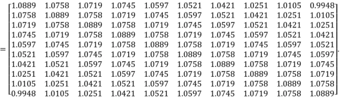
Also, the autovariance function 𝐾𝐾𝑥𝑥(𝑘𝑘, 𝑘𝑘) of the state vector 𝑥𝑥(𝑘𝑘) is calculated as 𝐾𝐾𝑥𝑥(𝑘𝑘, 𝑘𝑘) = ⎣ ⎢ ⎢ ⎢ ⎢ ⎢ ⎢ ⎢ ⎢ ⎡1.0889 1.0758 1.0719 1.0745 1.0597 1.0521 1.0421 1.0251 1.0105 0.9948_{1.0758 1.0889 1.0758 1.0719 1.0745 1.0597 1.0521 1.0421 1.0251 1.0105} 1.0719 1.0758 1.0889 1.0758 1.0719 1.0745 1.0597 1.0521 1.0421 1.0251 1.0745 1.0719 1.0758 1.0889 1.0758 1.0719 1.0745 1.0597 1.0521 1.0421 1.0597 1.0745 1.0719 1.0758 1.0889 1.0758 1.0719 1.0745 1.0597 1.0521 1.0521 1.0597 1.0745 1.0719 1.0758 1.0889 1.0758 1.0719 1.0745 1.0597 1.0421 1.0521 1.0597 1.0745 1.0719 1.0758 1.0889 1.0758 1.0719 1.0745 1.0251 1.0421 1.0521 1.0597 1.0745 1.0719 1.0758 1.0889 1.0758 1.0719 1.0105 1.0251 1.0421 1.0521 1.0597 1.0745 1.0719 1.0758 1.0889 1.0758 0.9948 1.0105 1.0251 1.0421 1.0521 1.0597 1.0745 1.0719 1.0758 1.0889⎦⎥ ⎥ ⎥ ⎥ ⎥ ⎥ ⎥ ⎥ ⎤ .

By substituting the system matrix Φ, the autovariance function 𝐾𝐾𝑥𝑥(𝑘𝑘, 𝑘𝑘) of the state vector, the

observation vector 𝐻𝐻 and the parameters 𝑎𝑎̄𝑖𝑖,𝑁𝑁, 𝑖𝑖 = 1, 2, ⋯ , 𝐿𝐿 + 1, in (19) into the fixed-lag

smoothing algorithm in Theorem 2, the RLS Wiener fixed-lag smoothing estimates 𝑧𝑧̂(𝑘𝑘 − 𝐿𝐿, 𝑘𝑘) of the signal 𝑧𝑧(𝑘𝑘 − 𝐿𝐿) are calculated recursively.

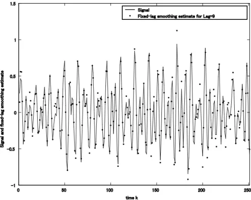
Fig. 1 Signal 𝑧𝑧(𝑘𝑘 − 9) and the fixed-lag smoothing estimate 𝑧𝑧̂(𝑘𝑘 − 9, 𝑘𝑘) by the RLS Wiener fixed-lag smoother in Theorem 2 vs. 𝑘𝑘, 10 ≤ 𝑘𝑘 ≤ 259, for 𝛷𝛷𝛷𝛷𝛷𝛷 = 10[𝑑𝑑𝐵𝐵].

(11)

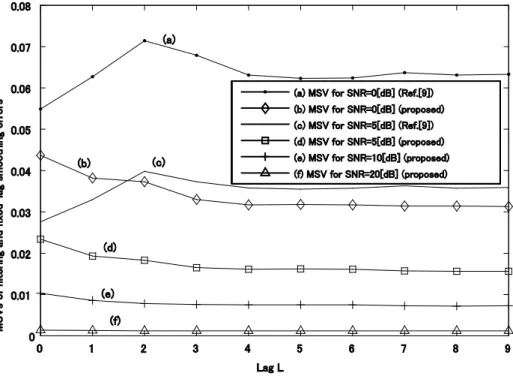
Fig.1 illustrates the signal 𝑧𝑧(𝑘𝑘 − 9) and the fixed-lag smoothing estimate 𝑧𝑧̂(𝑘𝑘 − 9, 𝑘𝑘) by the RLS Wiener fixed-lag smoother in Theorem 2 vs. 𝑘𝑘 , 10 ≤ 𝑘𝑘 ≤ 259 , for the signal-to-noise ratio 𝛷𝛷𝛷𝛷𝛷𝛷 = 10 [𝑑𝑑𝐵𝐵]. Fig.2 illustrates the mean-square values (MSVs) of the filtering and fixed-lag smoothing errors by the RLS Wiener fixed-lag smoother in Theorem 2 for 𝛷𝛷𝛷𝛷𝛷𝛷 = 0, 5, 10, 20[𝑑𝑑𝐵𝐵]. For 𝐿𝐿 = 0, the MSVs of the filtering errors are plotted. In Fig.2, particularly for 𝛷𝛷𝛷𝛷𝛷𝛷 = 0[𝑑𝑑𝐵𝐵] and 𝛷𝛷𝛷𝛷𝛷𝛷 = 5[𝑑𝑑𝐵𝐵], as the fixed lag 𝐿𝐿 increases, the MSVs of the fixed-lag smoothing errors decrease. For 𝛷𝛷𝛷𝛷𝛷𝛷 = 10[𝑑𝑑𝐵𝐵], as the fixed lag increases, the MSV of the fixed-lag smoothing errors decreases gradually. The larger the value of the 𝛷𝛷𝛷𝛷𝛷𝛷 becomes, the smaller the MSVs of the filtering and smoothing errors become. Under the same stochastic assumptions for the signal and the observation noise, for each value of the 𝛷𝛷𝛷𝛷𝛷𝛷, the fixed-lag smoothing estimates by the fixed-lag smoother [9] diverge.

Fig. 2 Mean-square values of the filtering and fixed-lag smoothing errors by the RLS Wiener fixed-lag smoother in Theorem 2 for 𝛷𝛷𝛷𝛷𝛷𝛷 = 0, 5, 10, 20[𝑑𝑑𝐵𝐵].

Here, the MSVs of the fixed-lag smoothing and filtering errors are evaluated by ∑1000+𝐿𝐿(

𝑘𝑘=𝐿𝐿+1 𝑧𝑧(𝑘𝑘 − 𝐿𝐿) −

𝑧𝑧̂(𝑘𝑘 − 𝐿𝐿, 𝑘𝑘))2_{/1000 and ∑}1000₍

(12)

6.2. Example 2

As the second example, let us adopt the sound signal ”Laughter” which is usable in the MATLAB program. The sampling frequency of the voice signal is 8.192 [kHz]. The autocovariance data of the signal is calculated in terms of 5,000 sampled signal data.

Suppose that the signal process is modeled in terms of the AR model of order 10 in (9). The 1 × 10 observation vector is expressed as (10). The state equation is given by (11). The parameters in the system matrix Φ are as follows:

𝑎𝑎1= −0.9372, 𝑎𝑎2= 0.9500, 𝑎𝑎3= −0.1625, 𝑎𝑎4= 0.4429, 𝑎𝑎5= −0.1555,

𝑎𝑎6= 0.3668, 𝑎𝑎7= 0.0207, 𝑎𝑎8= 0.3125, 𝑎𝑎9= −0.2216, 𝑎𝑎10= 0.3069.

Also, the autovariance function 𝐾𝐾𝑥𝑥(𝑘𝑘, 𝑘𝑘) of the state 𝑥𝑥(𝑘𝑘) is calculated as 𝐾𝐾𝑥𝑥(𝑘𝑘, 𝑘𝑘) = ⎣ ⎢ ⎢ ⎢ ⎢ ⎢ ⎢ ⎢ ⎢ ⎡ 0.1418_0.0800 0.0800 −0.0256 −0.0809 −0.0653 −0.0152_0.1418 _{0.0800 −0.0256 −0.0809 −0.0653 −0.0152}0.0148 0.0114 −0.0005 −0.0002_0.0148 _{0.0114 −0.0005} −0.0256 0.0800 0.1418 0.0800 −0.0256 −0.0809 −0.0653 −0.0152 0.0148 0.0114 −0.0809 −0.0256 0.0800 0.1418 0.0800 −0.0256 −0.0809 −0.0653 −0.0152 0.0148 −0.0653 −0.0809 −0.0256 0.0800 0.1418 0.0800 −0.0256 −0.0809 −0.0653 −0.0152 −0.0152 −0.0653 −0.0809 −0.0256 0.0800 0.1418 0.0800 −0.0256 −0.0809 −0.0653 0.0148 −0.0152 −0.0653 −0.0809 −0.0256 0.0800 0.1418 0.0800 −0.0256 −0.0809 0.0114 0.0148 −0.0152 −0.0653 −0.0809 −0.0256 0.0800 0.1418 0.0800 −0.0256 −0.0005 0.0114 0.0148 −0.0152 −0.0653 −0.0809 −0.0256 0.0800 0.1418 0.0800 −0.0002 −0.0005 0.0114 0.0148 −0.0152 −0.0653 −0.0809 −0.0256 0.0800 0.1418⎦⎥ ⎥ ⎥ ⎥ ⎥ ⎥ ⎥ ⎥ ⎤ .

By substituting the system matrix Φ, the autovariance function 𝐾𝐾𝑥𝑥(𝑘𝑘, 𝑘𝑘) of the state vector, the

bservation vector 𝐻𝐻 and the coefficients 𝑎𝑎̄𝑖𝑖,𝑁𝑁, 𝑖𝑖 = 1, 2, ⋯ , 𝐿𝐿 + 1, in (19) into the fixed-lag

smoothing algorithm in Theorem 2, the RLS Wiener fixed-lag smoothing estimates 𝑧𝑧̂(𝑘𝑘 − 𝐿𝐿, 𝑘𝑘) of the signal 𝑧𝑧(𝑘𝑘 − 𝐿𝐿) are calculated recursively.

(13)

Fig. 3 Signal 𝑧𝑧(𝑘𝑘 − 9) and the fixed-lag smoothing estimate 𝑧𝑧̂(𝑘𝑘 − 9, 𝑘𝑘) by the RLS Wiener fixed-lag smoother in Theorem 2 vs. 𝑘𝑘, 10 ≤ 𝑘𝑘 ≤ 259, for 𝛷𝛷𝛷𝛷𝛷𝛷 = 10[𝑑𝑑𝐵𝐵].

Fig.3 illustrates the signal 𝑧𝑧(𝑘𝑘 − 9) and the fixed-lag smoothing estimate 𝑧𝑧̂(𝑘𝑘 − 9, 𝑘𝑘) by the RLS Wiener fixed-lag smoother in Theorem 2 vs. 𝑘𝑘, 10 ≤ 𝑘𝑘 ≤ 259, for 𝛷𝛷𝛷𝛷𝛷𝛷 = 10 [𝑑𝑑𝐵𝐵]. Fig.4 illustrates

the MSVs of the filtering and fixed-lag smoothing errors by the RLS Wiener fixed-lag smoother in Theorem 2 for 𝛷𝛷𝛷𝛷𝛷𝛷 = 0, 5, 10, 20[𝑑𝑑𝐵𝐵] and the RLS Wiener fixed-lag smoother [9] for 𝛷𝛷𝛷𝛷𝛷𝛷 = 0, 5[𝑑𝑑𝐵𝐵]. For 𝐿𝐿 = 0, the MSVs of the filtering errors are plotted. In Fig.4, it is shown that the proposed RLS

Wiener fixed-lag smoother shows better estimation accuracy than the fixed-lag smoother [9]. For 𝛷𝛷𝛷𝛷𝛷𝛷 = 10[𝑑𝑑𝐵𝐵], the MSVs of the fixed-lag smoothing errors by the fixed-lag smoother [9] are fairly larger

than those by the proposed RLS Wiener fixed-lag smoother. Actually, these MSVs are 0.2704, 2.4815, 2.9695, 2.0858, 5.3556, 3.1665, 2.6676, 3.1021 and 2.7873 for 𝐿𝐿 = 0, 1, 2, ⋯ , 9.respectively.

(14)

Fig. 4 Mean-square values of the filtering and fixed-lag smoothing errors by the RLS Wiener fixed-lag

smoother in Theorem 2 for 𝛷𝛷𝛷𝛷𝛷𝛷 = 0, 5, 10, 20[𝑑𝑑𝐵𝐵] and the RLS Wiener fixed-lag smoother [9] for

𝛷𝛷𝛷𝛷𝛷𝛷 = 0, 5 [𝑑𝑑𝐵𝐵].

Here, the MSVs of the fixed-lag smoothing and filtering errors are evaluated by

∑

Ni+L

(z(k − L) − z�(k − L, k))

2

_/Ni

k=L+1

and ∑

Nk=1i

(z(k) − z�(k, k))

2

/Ni

, i = 1, 2 , respectively, where

N

1

= 1000 for the current fixed-lag smoother and N

2

= 250 for the previous fixed-lag smoother [9].

7. Conclusions

In this paper, the RLS fixed-lag smoother using the covariance information and the RLS Wiener fixed-lag

smoother have been newly devised in linear discrete-time wide-sense stationary stochastic systems.

In the proposed RLS Wiener fixed-lag smoother, for the signal process fitted to the AR model of order 𝛷𝛷,

the fixed-lag smoothing estimate 𝑧𝑧̂(𝑘𝑘 − 𝐿𝐿, 𝑘𝑘), 1 ≤ 𝐿𝐿 ≤ 𝛷𝛷 − 1, can be calculated. The key idea suggested

in the current approach is that the autocovariance function 𝐾𝐾(𝑘𝑘 − 𝐿𝐿, 𝑠𝑠) in the Wiener-Hopf equation is

expressed by (19) as the linear combination of 𝐾𝐾(𝑘𝑘, 𝑠𝑠) , 𝐾𝐾(𝑘𝑘 + 1, 𝑠𝑠) , ⋯ , 𝐾𝐾(𝑘𝑘 + 𝐿𝐿 − 1, 𝑠𝑠) and

𝐾𝐾(𝑘𝑘 + 𝐿𝐿, 𝑠𝑠).

In the numerical simulation examples, for the two kinds of stochastic signal processes, fitted to the AR

model of the order 𝛷𝛷 = 10, it has been shown that the proposed RLS Wiener fixed-lag smoother has the

stable and superior estimation characteristics in comparison with the fixed-lag smoother [9].

Fig. 4 Mean-square values of the filtering and fixed-lag smoothing errors by the RLS Wiener fixed-lag smoother in Theorem 2 for 𝛷𝛷𝛷𝛷𝛷𝛷 = 0, 5, 10, 20[𝑑𝑑𝐵𝐵] and the RLS Wiener fixed-lag smoother [9] for 𝛷𝛷𝛷𝛷𝛷𝛷 = 0, 5 [𝑑𝑑𝐵𝐵].

Here, the MSVs of the fixed-lag smoothing and filtering errors are evaluated by ∑ (z(k − L) − z�(k − L, k))2_/N

i Ni+L

k=L+1 and ∑Nk=1i (z(k) − z�(k, k))2/Ni, i = 1, 2 , respectively, where

N1= 1000 for the current fixed-lag smoother and N2= 250 for the previous fixed-lag smoother [9].

7. Conclusions

In this paper, the RLS fixed-lag smoother using the covariance information and the RLS Wiener fixed-lag smoother have been newly devised in linear discrete-time wide-sense stationary stochastic systems.

In the proposed RLS Wiener fixed-lag smoother, for the signal process fitted to the AR model of order 𝛷𝛷, the fixed-lag smoothing estimate 𝑧𝑧̂(𝑘𝑘 − 𝐿𝐿, 𝑘𝑘), 1 ≤ 𝐿𝐿 ≤ 𝛷𝛷 − 1, can be calculated. The key idea suggested in the current approach is that the autocovariance function 𝐾𝐾(𝑘𝑘 − 𝐿𝐿, 𝑠𝑠) in the Wiener-Hopf equation is expressed by (19) as the linear combination of 𝐾𝐾(𝑘𝑘, 𝑠𝑠) , 𝐾𝐾(𝑘𝑘 + 1, 𝑠𝑠) , ⋯ , 𝐾𝐾(𝑘𝑘 + 𝐿𝐿 − 1, 𝑠𝑠) and 𝐾𝐾(𝑘𝑘 + 𝐿𝐿, 𝑠𝑠).

In the numerical simulation examples, for the two kinds of stochastic signal processes, fitted to the AR model of the order 𝛷𝛷 = 10, it has been shown that the proposed RLS Wiener fixed-lag smoother has the stable and superior estimation characteristics in comparison with the fixed-lag smoother [9].

(15)

References

[1] J. B. Moore, Discrete-time fixed-lag smoothing algorithms, Automatica, 9 (1973), 163-173.

[2] H. E. Rauch, A new approach to linear filtering and prediction problem, IEEE Trans. Aut. Control, AC-8 (1963), 371-372.

[3] J. S. Meditch, Stochastic Optimal Linear Estimation, McGraw-Hill, New York, 1969.

[4] T. Kailath and P. Frost, An innovations approach to least-squares estimation: Part II-Linear smoothing in additive white noise. IEEE Trans. Aut. Control,. AC-13 (1968), 646-655.

[5] D. Simon, Optimal Sate Estimation, Wiley New York, 2006.

[6] S. Nakamori, M. Sugisaka, Design of linear fixed-lag smoother by covariance information, Trans. SICE 14 (4) (1978) 405–412.

[7] S. Nakamori, Recursive estimation technique of signal from output measurement data in linear discrete-time systems, IEICE Trans. Fund. Electron. Commun. Comput. Sci. E782-A (5) (1995) 600–607. [8] S. Nakamori, A. Hermoso-Carazo, J. Linares-Pe’rez, Design of RLS Wiener fixed-lag smoother using covariance information in linear discrete stochastic systems, Applied Mathematical Modelling, 32(7) (2008), 1338-1349.

[9] S. Nakamori, A. Hermoso-Carazo, J. Linares-Pe’rez, Design of fixed-lag smoother using covariance information based on innovations approach in linear discrete-time systems, 193(1), pp. 162-174, 2007. [10] S. Nakamori, A. Hermoso-Carazo, J. Linares-Pe’rez, Design of RLS fixed-lag smoother using covariance information in linear discrete stochastic systems, Applied Mathematical modeling, 34(4), 1093-1106, 2010.

[11] S. Nakamori, Design of recursive least-squares fixed-lag smoother using covariance information in linear continuous stochastic systems, Applied Mathematical Modelling, 31(8) (2007) 1609-1620.

[12] A.P. Sage, J.L. Melsa, Estimation Theory with Applications to Communications and Control, McGraw-Hill, New York, 1971.

Appendix 1 (Proof of Theorem 1)

Let us introduce the function 𝐽𝐽(𝑘𝑘, 𝑠𝑠), which satisfies 𝐽𝐽(𝑘𝑘, 𝑠𝑠)𝑅𝑅 = 𝐵𝐵𝑇𝑇_{(𝑠𝑠) − � 𝐽𝐽}

𝑘𝑘 𝑖𝑖=1

(𝑘𝑘, 𝑖𝑖)𝐾𝐾(𝑖𝑖, 𝑠𝑠). (A-1)

From (3), (8) and (19), it is seen that

ℎ(𝑘𝑘, 𝑠𝑠) = (𝑎𝑎̄1,𝐿𝐿𝐴𝐴(𝑘𝑘) + 𝑎𝑎̄2,𝐿𝐿𝐴𝐴(𝑘𝑘 + 1) + 𝑎𝑎̄3,𝐿𝐿𝐴𝐴(𝑘𝑘 + 2) + ⋯ + 𝑎𝑎̄𝑁𝑁,𝐿𝐿𝐴𝐴(𝑘𝑘 + 𝐿𝐿))𝐽𝐽(𝑘𝑘, 𝑠𝑠). (A-2)

(16)

(𝐽𝐽(𝑘𝑘, 𝑠𝑠) − 𝐽𝐽(𝑘𝑘 − 1, 𝑠𝑠))𝑅𝑅 = −𝐽𝐽(𝑘𝑘, 𝑘𝑘)𝐾𝐾(𝑘𝑘, 𝑠𝑠) − �(

𝑘𝑘−1 𝑖𝑖=1

𝐽𝐽(𝑘𝑘, 𝑖𝑖) − 𝐽𝐽(𝑘𝑘 − 1, 𝑠𝑠))𝐾𝐾(𝑖𝑖, 𝑠𝑠). (A-3) From (A-1) and (A-3), it follows that

𝐽𝐽(𝑘𝑘, 𝑠𝑠) − 𝐽𝐽(𝑘𝑘 − 1, 𝑠𝑠) = −𝐽𝐽(𝑘𝑘, 𝑘𝑘)𝐴𝐴(𝑘𝑘)𝐽𝐽(𝑘𝑘 − 1, 𝑠𝑠). (A-4) Substituting (A-2) into (4), we have

𝑧𝑧̂(𝑘𝑘 − 𝐿𝐿, 𝑘𝑘) = (𝑎𝑎̄1,𝐿𝐿𝐴𝐴(𝑘𝑘) + 𝑎𝑎̄2,𝐿𝐿𝐴𝐴(𝑘𝑘 + 1) + ⋯ + 𝑎𝑎̄𝑁𝑁,𝐿𝐿𝐴𝐴(𝑘𝑘 + 𝐿𝐿)) � 𝐽𝐽 𝑘𝑘 𝑖𝑖=1 (𝑘𝑘, 𝑖𝑖)𝑦𝑦(𝑖𝑖). (A-5) Introducing 𝑒𝑒(𝑘𝑘) = � 𝐽𝐽 𝑘𝑘 𝑖𝑖=1 (𝑘𝑘, 𝑖𝑖)𝑦𝑦(𝑖𝑖), (A-6) we obtain (20).

Subtracting the equation obtained by putting 𝑘𝑘 → 𝑘𝑘 − 1 in (A-6) from (A-6), we have 𝑒𝑒(𝑘𝑘) − 𝑒𝑒(𝑘𝑘 − 1) = 𝐽𝐽(𝑘𝑘, 𝑘𝑘)𝑦𝑦(𝑘𝑘) + �( 𝑘𝑘−1 𝑖𝑖=1 𝐽𝐽(𝑘𝑘, 𝑖𝑖) − 𝐽𝐽(𝑘𝑘 − 1, 𝑖𝑖))𝑦𝑦(𝑖𝑖) = 𝐽𝐽(𝑘𝑘, 𝑘𝑘)𝑦𝑦(𝑘𝑘) − 𝐽𝐽(𝑘𝑘, 𝑘𝑘)𝐴𝐴(𝑘𝑘) � 𝐽𝐽 𝑘𝑘−1 𝑖𝑖=1 (𝑘𝑘 − 1, 𝑖𝑖)𝑦𝑦(𝑖𝑖). (A-7)

Here, the initial condition on the difference equation for 𝑒𝑒(𝑘𝑘) at 𝑘𝑘 = 0 is given by 𝑒𝑒(0) = 0 from (A-6). From (A-6) and (A-7), (22) is obtained.

Putting 𝑠𝑠 = 𝑘𝑘 in (A-1), we have 𝐽𝐽(𝑘𝑘, 𝑘𝑘)𝑅𝑅 = 𝐵𝐵𝑇𝑇_{(𝑘𝑘) − � 𝐽𝐽} 𝑘𝑘 𝑖𝑖=1 (𝑘𝑘, 𝑖𝑖)𝐾𝐾(𝑖𝑖, 𝑘𝑘) = 𝐵𝐵𝑇𝑇_{(𝑘𝑘) − � 𝐽𝐽} 𝑘𝑘 𝑖𝑖=1 (𝑘𝑘, 𝑖𝑖)𝐵𝐵(𝑖𝑖)𝐴𝐴𝑇𝑇_(𝑘𝑘). (A-8)

Introducing the function 𝑟𝑟(𝑘𝑘) = � 𝐽𝐽 𝑘𝑘 𝑖𝑖=1 (𝑘𝑘, 𝑖𝑖)𝐵𝐵(𝑖𝑖), (A-9) (A-8) is written as 𝐽𝐽(𝑘𝑘, 𝑘𝑘)𝑅𝑅 = 𝐵𝐵𝑇𝑇_{(𝑘𝑘) − 𝑟𝑟(𝑘𝑘)𝐴𝐴}𝑇𝑇_(𝑘𝑘). _(A-10)

(17)

𝑟𝑟(𝑘𝑘) − 𝑟𝑟(𝑘𝑘 − 1) = 𝐽𝐽(𝑘𝑘, 𝑘𝑘)𝐵𝐵(𝑘𝑘) + �( 𝑘𝑘−1 𝑖𝑖=1 𝐽𝐽(𝑘𝑘, 𝑖𝑖) − 𝐽𝐽(𝑘𝑘 − 1, 𝑖𝑖))𝐵𝐵(𝑖𝑖) = 𝐽𝐽(𝑘𝑘, 𝑘𝑘)𝐵𝐵(𝑘𝑘) − 𝐽𝐽(𝑘𝑘, 𝑘𝑘)𝐴𝐴(𝑘𝑘)𝑟𝑟(𝑘𝑘 − 1). (A-11)

From (A-10) and (A-11), (24) is obtained. Here, the initial condition on the difference equation for 𝑟𝑟(𝑘𝑘) at 𝑘𝑘 = 0 is given by 𝑟𝑟(0) = 0 from (A-9).

(Q.E.D.) Appendix 2 (Proof of Theorem 2)

From (20) and (21), with the relation 𝐴𝐴(𝑘𝑘) = 𝐻𝐻Φ𝑘𝑘_{, it is seen that}

𝑧𝑧̂(𝑘𝑘 − 𝐿𝐿, 𝑘𝑘) = 𝑎𝑎̄1,𝐿𝐿𝐻𝐻Φ𝑘𝑘𝑒𝑒(𝑘𝑘) + 𝑎𝑎̄2,𝐿𝐿𝐻𝐻ΦΦ𝑘𝑘𝑒𝑒(𝑘𝑘) + ⋯ + 𝑎𝑎̄𝑁𝑁,𝐿𝐿𝐻𝐻ΦΦ𝑘𝑘+𝐿𝐿𝑒𝑒(𝑘𝑘)

= 𝑎𝑎̄1,𝐿𝐿𝐻𝐻𝑥𝑥�(𝑘𝑘, 𝑘𝑘) + 𝑎𝑎̄2,𝐿𝐿𝐻𝐻Φ𝑥𝑥�(𝑘𝑘, 𝑘𝑘) + ⋯ + 𝑎𝑎̄𝑁𝑁,𝐿𝐿𝐻𝐻Φ𝐿𝐿𝑥𝑥�(𝑘𝑘, 𝑘𝑘).

Here, the filtering estimate 𝑥𝑥�(𝑘𝑘, 𝑘𝑘) of the state vector 𝑥𝑥(𝑘𝑘) is given by 𝑥𝑥�(𝑘𝑘, 𝑘𝑘) = Φ𝑘𝑘_{𝑒𝑒(𝑘𝑘). Substitution}

of (22) into 𝑥𝑥�(𝑘𝑘, 𝑘𝑘) = Φ𝑘𝑘_{𝑒𝑒(𝑘𝑘) yields}

𝑥𝑥�(𝑘𝑘, 𝑘𝑘) = Φ𝑥𝑥�(𝑘𝑘 − 1, 𝑘𝑘 − 1) + Φ𝑘𝑘_{𝐽𝐽(𝑘𝑘, 𝑘𝑘)�𝑦𝑦(𝑘𝑘) − 𝐻𝐻Φ𝑥𝑥�(𝑘𝑘 − 1, 𝑘𝑘 − 1)�,}

𝑥𝑥�(0,0) = 0. (A-12)

Here, the initial condition on the difference equation for the filtering estimate 𝑥𝑥�(𝑘𝑘, 𝑘𝑘) at 𝑘𝑘 = 0 is given by 𝑥𝑥�(𝑘𝑘, 𝑘𝑘) = 0 from 𝑥𝑥�(𝑘𝑘, 𝑘𝑘) = Φ𝑘𝑘_{𝑒𝑒(𝑘𝑘) with (A-6). Putting the filter gain in (A-12) as 𝐺𝐺(𝑘𝑘) =}

Φ𝑘𝑘_{𝐽𝐽(𝑘𝑘, 𝑘𝑘), we obtain (26). From (24), 𝐽𝐽(𝑘𝑘, 𝑘𝑘) is given by}

𝐽𝐽(𝑘𝑘, 𝑘𝑘) = (𝐵𝐵𝑇𝑇_{(𝑘𝑘) − 𝑟𝑟(𝑘𝑘 − 1)𝐴𝐴}𝑇𝑇_{(𝑘𝑘))(𝑅𝑅 + 𝐻𝐻𝐾𝐾}_𝑥𝑥_{(𝑘𝑘, 𝑘𝑘)𝐻𝐻}𝑇𝑇_{− 𝐴𝐴(𝑘𝑘)𝑟𝑟(𝑘𝑘 − 1)𝐴𝐴}𝑇𝑇_(𝑘𝑘))−1_.

Putting 𝛷𝛷(𝑘𝑘) = 𝐴𝐴(𝑘𝑘)𝑟𝑟(𝑘𝑘)𝐴𝐴𝑇𝑇_{(𝑘𝑘) = Φ}𝑘𝑘_{𝑟𝑟(𝑘𝑘)(Φ}𝑇𝑇₎𝑘𝑘_{, the filter gain is expressed as}

𝐺𝐺(𝑘𝑘) = (𝐴𝐴(𝑘𝑘)𝐵𝐵𝑇𝑇_{(𝑘𝑘) − 𝐴𝐴(𝑘𝑘)𝑟𝑟(𝑘𝑘 − 1)𝐴𝐴}𝑇𝑇_{(𝑘𝑘))(𝑅𝑅 + 𝐻𝐻𝐾𝐾}

𝑥𝑥(𝑘𝑘, 𝑘𝑘)𝐻𝐻𝑇𝑇− 𝐴𝐴(𝑘𝑘)𝑟𝑟(𝑘𝑘 − 1)𝐴𝐴𝑇𝑇(𝑘𝑘))−1

= (𝐾𝐾(𝑘𝑘, 𝑘𝑘) − Φ𝛷𝛷(𝑘𝑘 − 1)Φ𝑇𝑇_{)(𝑅𝑅 + 𝐻𝐻𝐾𝐾}

𝑥𝑥(𝑘𝑘, 𝑘𝑘)𝐻𝐻𝑇𝑇− Φ𝛷𝛷(𝑘𝑘 − 1)Φ𝑇𝑇)−1.

Finally, substituting (23) into 𝛷𝛷(𝑘𝑘) = 𝐴𝐴(𝑘𝑘)𝑟𝑟(𝑘𝑘)𝐴𝐴𝑇𝑇_{(𝑘𝑘), we obtain}

𝛷𝛷(𝑘𝑘) = 𝐴𝐴(𝑘𝑘)(𝑟𝑟(𝑘𝑘 − 1) + 𝐽𝐽(𝑘𝑘, 𝑘𝑘)(𝐵𝐵(𝑘𝑘) − 𝐴𝐴(𝑘𝑘)𝑟𝑟(𝑘𝑘 − 1)))𝐴𝐴𝑇𝑇_(𝑘𝑘)

= Φ𝛷𝛷(𝑘𝑘 − 1)Φ𝑇𝑇_{+ 𝐺𝐺(𝑘𝑘)(𝐻𝐻𝐾𝐾}

𝑥𝑥(𝑘𝑘, 𝑘𝑘) − 𝐻𝐻Φ𝛷𝛷(𝑘𝑘 − 1)Φ𝑇𝑇).

Here, the initial condition on the difference equation for 𝛷𝛷(𝑘𝑘) at 𝑘𝑘 = 0 is given by 𝛷𝛷(0) = 0 from 𝛷𝛷(𝑘𝑘) = 𝐴𝐴(𝑘𝑘)𝑟𝑟(𝑘𝑘)𝐴𝐴𝑇𝑇_{(𝑘𝑘) with (A-9).} _(Q.E.D.)