佐賀大学機関リポジトリ

Analysis on the Vibratory Characteristics

of A Vibroflot Beam

March 2005

Science and Technology of Energy

Department of Energy and Material Science

Graduate School of Science and Engineering

Saga University

Analysis on the Vibratory Characteristics

of a Vibroflot Beam

LiQiang, WANG

A dissertation submitted for the degree of

Doctor of Philosophy in Engineering

Science and Technology of Energy

Division of Energy and Material Science

Graduate School of Science and Engineering

Saga University

Submitted to Saga University

March 2005

Contents

Abstract

Chapter1. Background of research

1.1 Introductions···

···

···1

1.2 Soil improvement···

···

···1

1.2.1. Soft ground···

··

···1

1.2.2. Soil improvement···

··

···2

1.2.3. Purpose of soil improvement···

···

····3

1.3. Vibroflot···

··

·4

1.4. Objectives···

··

··7

1.5 Scope of the thesis···

··

·

··

9

1.6 References···

···

···10

Chapter2 Experimental Apparatus

2.1 Introduction···14

2.2. Working models···14

2.3 Experiment method···19

2.3.1. Experiment by strain gauge···19

2.3.2. Experiment by a high speed video camera···20

2.4 Conclusions···21

2.5 References···21

Chapter3. The pendulous motion analysis 3.1 Introduction ···

···

····22

3.2. Analysis of free pendulous vibration ···22

3.4 Calculation of inertia moment to the gravity center···27

3.5 Result of the two-degree pendulum···27

3.6 Conclusion ···

···

···29

3.7 References ···

···

···29

Chapter4. Analysis and Experiment of Free Vibration

4.1 Introduction ···

···

···30 4.2 Analytical Method ···

···

···30 4.3 Experimental Results ···

···

···39 4.3.1 Results of experiments ···39 4.3.2 Comparison ···

···

···48 4.4 Conclusions ···

···

···54 4.5 References ···

···

···55

Chapter5. Analysis an Experiment of Forced Vibration

5.1 Introduction ···

···

···56

5.2 Analytical method ···

···

···56

5.2.1 Normal Forced Vibration ···57

5.2.2 Amplitude Measurement ···59

5.3 Results and Discussion ···

···

···60

5.3.1 Free vibration ···

···

···61

5.3.2 Normal Forced Vibration ···65

5.4. Observation of forced vibration by a high speed video camera

···

···82

5.5 Conclusions ···

···

···87

Chapter6. Conclusions

6.1 Conclusions ···

···

···

···

···89

6.2 The work in the future ···

···

···90

Acknowledgement ···

···

···92

List of Figures and Tables

Figures

Fig.1-1. Schematic diagram of the equipment and process of soil

densification using vibroflotation technique ···5

Fig.1-2. Densified zones resulting from vibroflotation ···5

Fig.1-3. Displacement amplitudes of vibrator unit ···6

Fig.1-4. Illustration of the horizontal impacting forces and torsional shear induced by the vibroflot.··· ···6

Fig.1-5. Range of particle-size distributions suitable for densification by vibroflotation···7

Fig.2-1. A moving state of a working vibroflot ···14

Fig.2-2. A simplified state of a working vibroflot motion ···15

Fig.2-3 the model of simplify ···15

Fig.2-4 the process of simplify for a vibroflot ···16

Fig.2-5. the measured beam t ···16

Fig.2-6. the experimental installation ···17

Fig.2-7. the photo of the rectangular working model ···17

Fig.2-8. the cylindrical working model ···18

Fig.2-9. the cylinder of the cylindrical working model ···18

Fig.2-10. the photo of the cylindrical working model ···19

Fig.2-11. Experimental System by strain gauges ···19

Fig.3-1. the model of the pendulous motion···22 Fig.3-2 the calculation model of the center of gravity ……….………26

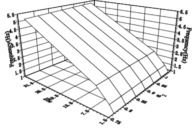
Fig.4-1. Coordinate system for theoretical analysis ···31 Fig.4-2. 3D-diagram of the relation among the first calculated natural frequency,

the rope length and the bottom mass in the case of that the plate thickness is 1mm.···41 Fig.4-3. 3D-diagram of the relation among the first measured natural frequency,

the rope length and the bottom mass in the case of that the plate thickness is 1mm ··

···

···41

Fig.4-4. 3D-diagram of the relation among the second calculated natural frequency,

the rope length and the bottom mass in the case of that the plate thickness is 1mm ··

···

···41

Fig.4-5. 3D-diagram of the relation among the second measured natural frequency,

the rope length and the bottom mass in the case of that the plate thickness is 1mm ··

···

···42

Fig.4-6. 3D-diagram of the relation among the first calculated natural frequency,

the rope length and the bottom mass in the case of that the plate thickness is 2mm ··

···

···44 Fig.4-7. 3D-diagram of the relation among the first measure natural frequency,

the rope length and the bottom mass in the case of that the plate thickness is 2mm. ··

···

····45

Fig.4-8. 3D-diagram of the relation among the second calculated natural frequency,

the rope length and the bottom mass in the case of that the plate thickness is 2mm ··

···

···45

Fig.4-9. 3D-diagram of the relation among the second measured natural frequency,

the rope length and the bottom mass in the case of that the plate thickness is 2mm ··

···

···46

Fig.4-10. 3D-diagram of the relation among the first calculated natural frequency,

the rope length and the bottom mass in the case of that the plate thickness is 3mm. ··

···

····47 Fig.4-11. 3D-diagram of the relation among the first measured natural frequency,

Fig.4-12. 3D-diagram of the relation among the second calculated natural frequency,

the rope length and the bottom mass in the case of that the plate thickness is 3mm. ··

···

····47

Fig.4-13. 3D-diagram of the relation among the second measured natural frequency,

the rope length and the bottom mass in the case of that the plate thickness is 3mm ··

···

···48

Fig.4-14. Comparison between 1st calculated and measured frequency by rope length 5mm with calculated and measured results of support-free

condition at the plate thickness 1mm ···51 Fig.4-15. Comparison between 1st calculated and measured frequency by

rope length 5mm with calculated and measured results of support-free

condition at the plate thickness 2mm ···51 Fig.4-16. Comparison between 1st calculated and measured frequency by

rope length 5mm with calculated and measured results of support-free

condition at the plate thickness 3mm ···51 Fig.4-17. Comparison between 2nd calculated and measured frequency by

rope length 500mm with calculated results of support-free

condition at the plate thickness 1mm ···52 Fig.4-18. Comparison between 2nd calculated and measured frequency by

rope length 500mm with calculated results of support-free

condition at the plate thickness 2mm ···52 Fig.4-19. Comparison between 2nd calculated and measured frequency by

rope length 500mm with calculated results of support-free

condition at the plate thickness 3mm ···52

Fig.5-2. 3D-diagram of the relation among calculated first natural frequency,

the wire length and the mass of the eccentricity rotor ···63

Fig.5-3. 3D-diagram of the relation among measured first natural frequency, the wire length and the mass of the eccentricity rotor ···64

Fig.5-4. 3D-diagram of the relation among calculated second natural frequency, the wire length and the mass of the eccentricity rotor ···64

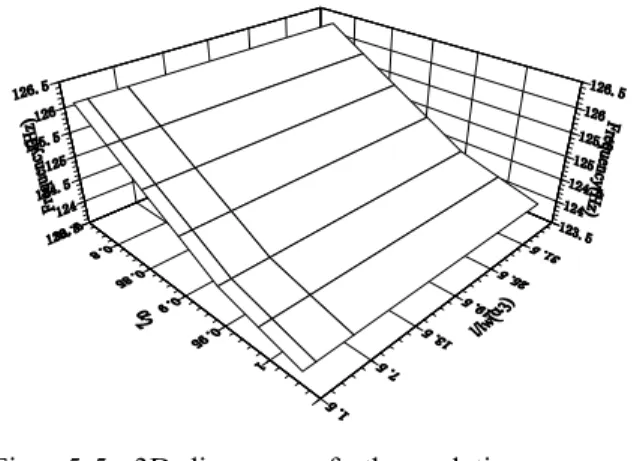
Fig.5-5. 3D-diagram of the relation among measured second natural frequency, the wire length and the mass of the eccentricity rotor ···64

Fig.5-6. the calculated moment, lw=20mm. ···66

Fig.5-7. the measured moment, lw=20mm. ···

···

···66

Fig.5-8. the calculated amplitude, lw=20mm. ···

···

···66

Fig.5-9. the calculated moment, lw=100mm . ···

···

···67

Fig.5-10. the measured moment, lw=100mm. ···

···

···67

Fig.5-11. the calculated amplitude, lw=100mm. ···

···

···67

Fig.5-12. the calculated moment, lw=250mm. ···

···

···70

Fig.5-13. the measured moment, lw=250mm. ···

···

···70

Fig.5-14. the calculated amplitude, lw=250mm. ···

···

···70

Fig.5-15. the calculated moment, lw=500mm. ···

···

···71

Fig.5-16. the measured moment, lw=500mm. ···

···

···71

Fig.5-17. the calculated amplitude, lw=500mm. ···

···

···71

Fig.5-18. the calculated moment, α2=0.813. ···

·

·73

Fig.5-19. the measured moment, α2=0.813. ···

·

·73

Fig.5-21. the calculated moment,α2=0.857. ···

·

·74

Fig.5-22. the measured moment, α2=0.867. ···

·

·74

Fig.5-23. the calculated amplitude, α2=0.867 ···

·

·74

Fig.5-24. Calculated moment, α2=0.901. ···

·

·76

Fig.5-25. Measured moment, α2=0.901. ···

·

·76

Fig.5-26. the calculated amplitude, α2=0.901. ···

·

·76

Fig.5-27. Calculated moment, α2=0.945. ···

·

·77

Fig.5-28. Measured moment, α2=0.945. ···

·

·77

Fig.5-29. the calculated amplitude, α2=0.945. ···

·

·77

Fig.5-30. Calculated moment, α2=0.989. ···

·

·79

Fig.5-31. Measured moment, α2=0.989. ···

·

·79

Fig.5-32. the calculated amplitude, α2=0.989. ···

·

·79

Fig.5-33. Calculated moment, α2=1.033. ···80

Fig.5-34. Measured moment, α2=1.033.··· ···

·

···80

Fig.5-35. the calculated amplitude, α2=1.033. ···

·

·80

Fig. 5-36 Photos of forced vibration as lw=100mm···

·

·82, 83

Fig.5-37 the photos of the top measured points as the different eccentricity rotor load

in the case of the hanging wire length is 100mm and 500mm.···

·

·84, 85

Fig. 5-38 the photos of the bottom measured points as the different eccentricity rotor load

Tables

Table 3-1 Calculation gravity center position under the experiment conditions ···27

Table 3-2 Calculated inertia moments to the gravity center ···27

Table 3-3 First frequency of the two-degree pendulum as lr=170mm. ···28

Table 3-5 Second frequency of the two-degree pendulum as lr=170mm ···28

Table 3-4 First frequency of the two-degree pendulum as lr=120mm. ···29

Table 3-5 Second frequency of the two-degree pendulum as lr=120mm. ···29

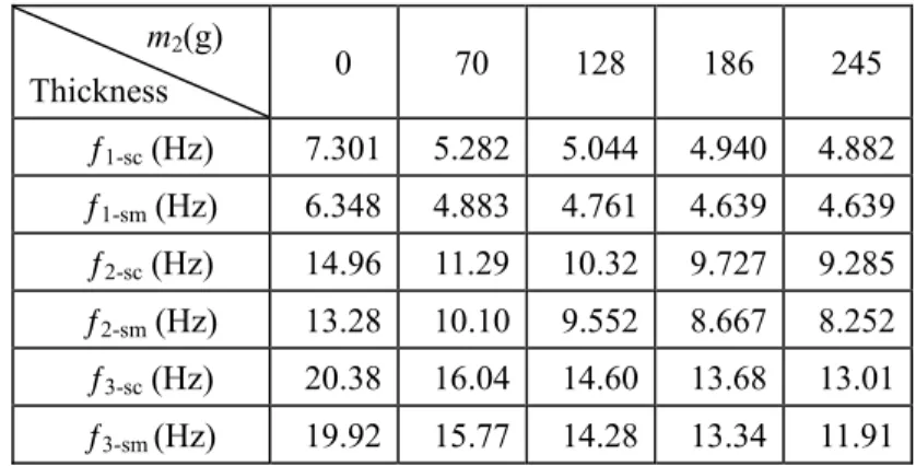
Table 4-1 List of parameters used for the calculations and the measurements. ··

····

···

··

39

Table 4-2 Results of calculation and measurement of simple support-free condition. ···48

Table4-3 Results of calculation of free-free condition. ···53

Abstract

A vibratory machine (vibroflot) is used for solidifying ground, which consists of a

cylindrical beam, a motor and an eccentricity rotor. The motor and the eccentricity rotor are

attached to the top and bottom of the cylindrical beam, respectively, linked though a central

axis. During a working process, the turning eccentricity rotor results in the vibration of the

cylindrical beam of vibroflot.

In order to analyze the beam vibration of the vibroflot, a theoretical model has been

proposed which was built on the basis of a rectangular model. The working model consists

of a rectangular steel plate suspended from a supporting bar through a thin cloth and

variable masses were attached to the bottom and to the top of the steel plate. Using this

working model, the effects of the weight of top mass and bottom mass, the thickness of the

steel plate, as well as the length of the suspending cloth have been systematically

investigated. The experimental results agreed satisfactorily with the theoretical prediction.

Using the rectangular working model, although the experimental results are consistent

well with the theoretical prediction, it was pained that the beam of the practical machine is

a cylinder, which is different with the rectangular beam. Therefore, the rectangular working

model was revised using a cylindrical beam instead of rectangular steel plate beam in order

to go a step further prove that our theoretical model applies the vibrational analysis of

vibroflot in general case.

The new working model consists of a suspended cylindrical beam connected with a

supporting bar though a wire, a motor and an eccentricity rotor, which were attached to the

top and bottom of the cylinder through a central axis. Using our theoretical model to deal

with the new working model, the experimental results are consistent well theoretical

Chapter 1

Background of research

1.1. Introduction

Vibroflot is a device using physical soil improvement, which is often efficient in stabilizing the soft cohesionless soils (sandy soils) by the vibration stabilization techniques. The physical method called vibroflotation method[Ref.1~13], in which the vibration of a vibroflot beam is utilized to improve the soft cohesionless soils (sandy soils). Since the vibration of a vibroflot beam provides the power for soil improvement, thus the vibratory characteristics of a vibroflot beam are necessary to investigate. This research is an experimental analysis about the vibratory characteristic of a vibroflot beam in order to guide the designing calculation for the company of the manufacturing vibroflot. The present theoretical analysis is experimentally verified and can be more accurately calculate the natural frequency than the method that is used in company now. The rotation speed of motor should be more accurately chosen in order to get larger amplitude to work and be kept away from dangerous resonance. Thus the vibratory characteristics of vibroflot beam are the objectives of the present research.

In this chapter, some information of soil improvement and vibroflot are explained. The status quo of research is also introduced about the vibration of a beam, and the reason is explained why the present research is chosen.

1.2. Soil improvement

It is known that the bearing capacity of the buildings is come from the foundation, so the characteristic of ground must be investigated before the construction work start. In general case, the soft ground always will be improved from the viewpoint of the safety of the upper buildings. So the soil improvement and soft ground est. are simply introduced later.

1.2.1. Soft ground

The ingredient of the soil that consists of ground particle, water and air, and it influences the characteristic of ground.

In foundation investigation, the soft ground is often judged by bearing capacity of soil. In general, the ground was called soft ground, which the bearing capacity is less than 3 tons/m2 (standard from Incorporated company BOK, Japan).

The soft ground is also divided two types by the characteristics of soil, soft cohesion soils and soft cohesionless soils. The soft cohesive soil means a soil that when unconfined has considerable strength when air-dried and that has significant cohesion when submerged, and the soft cohesiveless soil (sandy soil) means a soil that when unconfined has little or no strength when air-dried and that has little or no cohesion when submerged.

31% of continental area on our earth is sandy soil or desert, with a total area amounting to 48,000,000 km2. While the world population continuously increasing, the arable area is ceaselessly decreasing due to expanding of deserts.

Densification of the soft cohesionless soils (sandy soil) is carried out using shock and vibration. Vibroflotation is used to improve poor foundations. The process may decreasesettlement by more than 50% and the shearing strength of treated soils is increases substantially. Vibrations can convert loosely packed soils into a denser state.

1.2.2. Soil improvement Soil improvement

Soil improvement is a process that makes the density of ground becomes larger, the ratios of water

and air decreases; and make the ground strong to improve the ability of bearing capacity of soil.

Methods of soil improvement

The methods of soil improvement have four types based on the effect characteristics such as physic, chemistry, biology and heating.

a). Chemical method

The chemistry method of ground improvement is a process that the ground is instilled the chemical martial such as cement and lime, which make a chemical reaction with the water or air. The products of the reaction contact with the ground particle, and decrease the ratios of the water and the air. Thus

the density of ground was improved. b). Heat method

Heating to higher temperatures can result in significant permanent property improvements, including decreases in water sensitivity, swelling, and compressibility; and increases in strength. Dry or partly saturated weak clayey soils and loess are well suited for this type of treatment, which is presently regarded as experimental.

c). Biology method

The biology method is a ground improvement method that was developed recently. It often use a vegetation method to slope part which is the only practical biology method for soil improves

d). Physic method

The physic method of ground improvement is a method that based on a physical action such as substitution, bundle hardening, and reinforcement, to improve the foundation.

In the physic method, the soil improvement has many method of construction by the work form. Such as the replacing method, the high-densities method and the draining method, all of them are the physic method. The vibroflot machine is used for making the foundation to high-densities, which is studying at present.

Influence on sandy soil improvement

To the process of soil improvement, the influence factors on soil improvement are given as follows. 1. The size of soil particle

2. The size of filling martial 3. The permeability

4. The relative void ratio of the soil

1.2.3. Purpose of soil improvement

a) Improve liquefaction intensity

The factor of safety against liquefaction (FS), as defined in this thesis, is the ratio of Capacity to Demand. To increase FS, the Capacity of the soil can be increases, the Demand imposed on the soil

can be decreases, or both the Capacity and Demand can changed (increases or decreased) in such a way that there is a net increase in their ratio.

b) Decreases land subsidence

Land subsidence is the lowering of the land-surface elevation from changes that take place underground. Common causes of land subsidence from human activity are pumping water, oil, and gas from underground reservoirs; dissolution of limestone aquifers (sinkholes); collapse of underground mines; drainage of organic soils; and initial wetting of dry soils.

c) Improve the support power and the building stability.

The support power and the building stability are clearly important to the building of the ground surface. If they were not strong, the building would be easy to be destroyed by the external force such as earthquake or the weight of itself.

1.3. Vibroflot

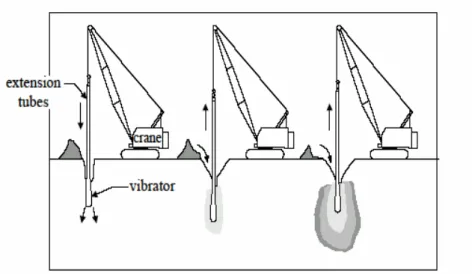
The vibroflot consists of a cylindrical beam, a motor and an eccentricity rotor, and it is hung though a wire by a crane in working. The motor and the eccentricity rotor are attached to the top and bottom of the cylindrical beam, respectively, linked through a central axis. During a working process (Fig.1-4), the turning eccentricity rotor results in the vibration of the cylindrical beam of vibroflot.

The vibroflot is used to make a cylindrical, vertical hole under its own weight by jetting to the desired depth. Then, 1/2- to 1- cubic yard coarse granular backfill, usually gravel or crushed rock 3/4 to 1 inch is dumped in, and the vibroflot is used to compact the gravel vertically and radically into the surrounding soft soil. The process of backfilling and compaction by vibration is continued until the densified stone column reaches the surface.

Vibroflotion method is presently considered to be one of the premier methods for densifying deep

sand deposits. The combined vibrator and extension tubes are referred to as the vibroflot. A schematic diagram of the Eq.ipment and process is given in Figure 1-1. As depicted in this figure, the vibroflot is usually jetted into the ground to the desired depth of improvement. The soil densities during withdrawal of the vibroflot as a result of lateral and torsional vibrations while the vibroflot is

repeatedly inserted and withdrawn in about 1m increments. The cavity that forms at the surface is backfilled with sand or gravel to form a column of densified soil (Mitchell and Gallagher 1998). The anatomy of a densities zone is further illustrated in Figure 1-2. The displacement amplitudes are shown in Fig1-3.

Figure 1-1. Schematic diagram of the Eq.ipment and process of soil densification using vibroflotation technique. (Adapted from Hayward Baker 1996).

A: Cylinder of compacted material added from the surface to compensate for the loss of volume caused by the increase of density of the compacted soil.

B. Cylinder of compacted material for a single compaction point.

Figure 1-2. Densified zones resulting from vibroflotation.

(Adapted from Brown 1977).

The interaction of the vibroflot and the surrounding soil is very complex, especially when water and backfill are introduced into the borehole during vibration. A conceptual illustration of the interaction

and the induced stresses and strains on the surrounding soil is shown in Figure 1-4.

Fig.1-3. Displacement amplitudes of vibrator unit

Figure 1-4. Illustration of the horizontal impacting forces and torsional shear induced by the vibroflot. (Adapted from Greenwood 1991).

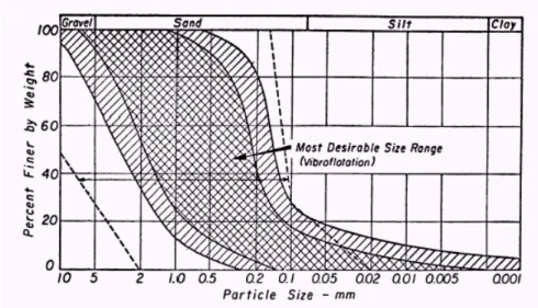
Figure 1-5. Range of particle-size distributions suitable for densification

(Courtesy of J. K. Mitchell, "Innovations in Ground Stabilization," Chicago Soil Mechanics Lecture Series, Innovations in Foundation Construction, Illinois Section, 1972. Reprinted by permission of The American Society of Civil Engineers, New York.)

The approximate variation of the post-treated relative density as a function of the tributary area per compaction point and soil type is shown in Figure 1-5. Although this figure may be used to select the initial spacing of the compaction points, field tests should be performed to finalize the design.

1.4. Objectives

In the front, the vibroflot and the information of soft ground and soil improvement were introduced; this is not the objective of the present research. Although the vibroflot is introduced in [Ref.14-22], the scope of the research was limited to geotechnics. The objective of the present research is classification of the vibratory characteristics of a vibroflot beam.

Mizoda Company (Japan) had designed and manufactured the vibroflot with an 8 m long beam. In their designing calculation, the vibrated speed of an inertia wheel of cylindrical beam was calculated by a method that is a half of the natural frequency’s sum of the free-free boundary conditions and the fixed-free boundary conditions. The relationship between the natural frequencies and the structural

parameters such as the length of the hanging wire, the weight of the eccentricity rotor, and the weight of a motor, the cylindrical beam length, and a cylindrical cross-sectional area etc., were not investigated. Thus using this method, the natural frequency can not be accurately calculated. To a vibroflot, one hand we need to choose the rotation speed of a motor to keep away from the natural frequency that is dangerous for resonance, on the other hand we try to choose the rotation speed of motor to approach the range of resonance in order to get larger amplitude to work. Thus the hanging beam’s natural frequency of the vibroflot needs to be accurately calculated.

Although the researches about beam were introduced using different methods or different form under the different really situations in journals[22-41], from machinery dynamics of view, these researches can be summarized to five types, the free-free boundary conditions[22,27], the fixed-fixed boundary condition[27,36-41], the fixed-free boundary condition[22,27-35], the simply support-free boundary conditions[25,26,27] and support-support boundary conditions[22-24,27].

G. R. LIU AND T. Y. WU [Ref.22] had studied a straight Euler beam which had stepped cross-section only at one place under the Four types of boundary conditions (pinned, clamped, free an sliding).

Chen and Tan [Ref.23] performed a research of an elastically supported-supported beam which has a moving oscillator on the upper surface. And Ref 14 shows a simply support-free condition beam, which has a moving mass, Ref.27, 39 and 41 given the researches of a supported-supported beam, which has one or two mass in different positions.

Ref.25 and 31 shows vibration analysis of a rotating beam. And Ref.35 had given a discussion of an elastic beam, which was fixed on a moving cart and carrying a concentrated or moving mass.

Although the beam vibration in these researches is well discussed, the present boundary condition of a vibroflot beam is different with the boundary condition of above researches. The present boundary condition is a variable boundary condition. The boundary condition is varied between the simply support-free boundary condition and the free-free boundary condition. The effect factor is the length of the hanging wire; the vibration will simulate simply support-free boundary condition, as the length of

the hanging wire is very short; otherwise the vibration will follow the free-free boundary condition. So a theoretical analysis model is proposed and then the relationship of vibrational characterizes of the vibroflot beam with above mentioned 5 parameters were studied. The analysis is experimentally verified using a rectangular and a cylindrical working model.

Using the rectangular working model, the relationship between the natural frequency and the effects of the length of the hanging rope, the thickness of plate (area of cross-section) and the bottom load were theoretically and experimentally investigated

And in order to investigate the relationship between the amplitude and bottom load, hanging rope length in the forced vibration, the cylindrical working model of a vibroflot is designed. This cylindrical working model is more similar to a practical vibroflot and easy to deduce the information of a practical vibroflot.

The purpose of this research is to develop the theoretical analysis method and to verify it experimentally.

The details of the objectives are as follows.

A) A theoretical model is developed and the relationship of vibrational characterizes of the vibroflot with above mentioned 5 parameters are studied

B) The present theoretical model is experimentally verified in the case the free lateral vibration using a rectangular working model.

C) The present theoretical model is experimentally verified in the case the free lateral vibration and forced lateral vibration using a cylindrical working model.

1.5. Scope of the thesis

This thesis includes the following contents:

Chapter 1 gives an introduction about research background, and explains the reason for choosing this project. After that the object of the research is shown.

Chapter 2 will introduce the working models of a vibroflot that are used in experiments in order to obtain the information of a vibroflot. Then the working model and the experimental method will be

explained.

Chapter 3 will introduce a detail of the pendulous vibration analysis, which is necessary because the two-degree pendulous vibration always take place when the beam is vibrating in the lateral vibration. The theoretical model of two-degree vibration, the theoretical analysis method, the calculated results and results of discussion will all be shown in this section.

Chapter 4 will show the details of the analysis and experimental results of the free lateral vibration based on a rectangular working model. The larger influence coefficient of the hanging rope or wire length can be obtained by the rectangular working model. That can experimentally verify a view of the present theoretical analysis. Following the theoretical analysis, the lateral vibration will tend to the vibration of the simply support-free boundary conditions, as the influence coefficient of the hanging rope or wire length is comparatively large. This is a reason why not directly using a cylindrical working model. In this chapter, the theoretical model of the free lateral vibration, the theoretical analysis method, the results of calculation and experiment, and results of discussion will all be introduced. Some conclusions will be obtained there.

Chapter 5 will give a research about the analysis and experiment based on a cylindrical working model. In order to verify present theoretical analysis that was done in chapter 4, it is or not applied to the cylindrical working model, the experiment of free lateral vibration is done again. The calculated and measured results of free lateral vibration are also given and discussed.

And the theoretical analysis method of the forced lateral vibration is introduced too based on the cylindrical working model in this chapter. The results of calculation and experiment, and then discussion on the forced lateral vibration are also shown in this section. Some conclusions will be obtained there.

Chapter 6 will give the conclusions of this research until now based on the calculated and measured results of the free and forced lateral vibration. And the works of this reach in future is introduced.

1.6. References

(2). 土質工学会, 地盤改良の調査設計から施工まで, 三美印刷株式会社, ISBN4-8864-502-0 (3). Engineer Manual No. 1110-1-1905, U.S. Army Corps of Engineers 1992 P0-137

(4). Baez, J. I.: A design model for the reduction of soil liquefaction by Vibro Stone Columns, Dissertation, University of Southern California, 1995

(5). ENEL C.R.I.S.: Milano, 1991

(6). Covil, C.S., et al.: Case History: Ground treatment of the sandfill at the new airport at Chek Lap Kok, Hong

(7). Kong: Proc. 3rd. Intl. Conf. on Ground Improvement Geosystems, pp. 148-156, London, 1997 (8). Balkema, Rotterdam: Building on soft soils, Centre for Civil Engineering Research and Codes,

1996

(9). J.-M., Sims, M.: Vibroflotation in reclamations in Hong Kong, Ground Imporvement, 1, pp. 127-145, 1997

(10). Whitman; Soil Mechanics, John Wiley & Sons, New York, 1969

(11). H. J.: The design of vibro replacement, Ground Engineering, London, Dec. 1995

(12). H. J.: Vibro Replacement to prevent earthquake induced liquefaction, Ground Engineering, London, September 1998

(13). W.F. Soil Improvement Techniques and their Evolution, Balkema, Rotterdam, 1989

(14). Vibro Systems Inc., Vibratory Ground Improvement Manual, METHOD STATEMENT FOR VIBRO COMPACTION

(15). TM 5-818-1 / AFM 88-3, Chap. 16

(16). Civil Engineering Office, Civil Engineering Department, Hong Kong, The Government of the Hong Kong Special Administrative RegionFirst published, July 2003

(17). Mouhamadou Diakhate, The organic soil around the Seattle Arboretum By Mouhamadou Diakhate, Foundation Design in organic soils.

(18). Thomas S. Lee1, Thomas Jackson1, and Randy R. Anderson2: Innovative Designs of Seismic Retrofitting the Posey & Webster Street Tubes, Oakland/Alameda, California

(19). PORT WORKS DESIGN MANUAL, PART 3

(20).David J. White, Aaron Gaul, and Kenneth Hoevelkamp: HIGHWAY APPLICATIONS FOR RAMMED AGGREGATE PIERS IN IOWA SOILS, Iowa DOT Project TR-443 CTRE Project 00-60, Department of Civil and Construction Engineering

HANDBOOK, MIL-HDBK-1007/3 15 NOVEMBER 1997.

(22). G. R. LIU AND T. Y. WU: Vibration Analysis of Beams Using The Generalized Differential Quadrature Rule And Domain Decomposition, Journal of Sound and Vibration (2001), 246(3), 461-481

(23). Yonghong Chen, C. A. Tan and L. A. Bergman: Effects of Boundary Flexibility on the Vibration of a Continuum With a Moving Oscillator, Journal of Vibration and Acoustics, OCT. 2002, Vol. 124 / 552-560

(24). T.P. CHANG and C.-Y. CHANG, Vibration Analysis of Beams With a Two Degree-of-freedom Spring-Mass System, lnt. J. Solids Structures Vol. 35, Nos. 5~6, pp. 383~401, 1998

(25). M. D. Al-Ansary: Flexural vibrations of rotating beams considering rotary inertia, Computers and Structures 69 (1998) 321-328

(26). T. G. CHONDROS, A. D. DIMAROGONAS and J. YAO: Vibration of a Beam with a Breathing Crack, Journal of Sound and vibration (2001) 239(1), 57-67

(27). I. K. SILVERMAN, Flexural Vibrations of Circular Beams, Journal of Sound and Vibration, (1998), 210(5). 661-672

(28). M.-Y. Kim and N.-I. Kim: Analytical And Numerical Study on Spatial Free Vibration of Non-symmetric Thin-walled Curved beams, Journal of Sound and Vibration (2002) 258(4), 595-618

(29). Carlos M. Tiago, Vitor M. A. Leit˜ao: Analysis of free vibration problems with the Element-Free Galerkin method, Numerical Methods in Continuum Mechanics 2003, Zilina, Slovak Republic

(30). R. V. Field, Jr., a L. A. Bergman & W. Brenton Hall b: Computation of probabilistic stability measures for a controlled distributed parameter system, Probabilistic Engineering Mechanics 10 (1995) 181-192

(31). K. H. LOW and MICHAEL W. S. LAU: Experimental Investigation of the Boundary Condition of Slewing Beams Using a High-speed Camera System, Mech. Math. Theory Vol. 30, No. 4, pp. 629-643, 1995

(32). F. W. WILLIAMS, S. YUAN AND K. YE, D. KENNEDY AND M. S. DJOUDI: Towards Deep and Simple Understanding of the Transcendental Eigenproblem of Structural Vibrations, Journal of Sound and Vibration (2002), 256(4), 681-693

carrying a moving mass, International Journal of Non-Linear Mechanics 38 (2003) 1481 – 1493

(34). W. W. WHITEMAN: Multi-Mode Analysis of Beam-Like Structures Subjected to Displacement Dependent Dry Friction Damping, Journal of Sound and Vibration, (1997), 207(3), 403-418

(35). S. PARK, B. K. KIM AND Y. YOUM: Single-Mode Vibration Suppression For a Beam-mass-cart System Using Input Preshaping With a Robust Internal-Loop Compensator, Journal of Sound and vibration (2001) 241(4), 693-716

(36). A. ARPACI, Annular Plate Dampers Attached To Continuous Systems, Journal of Sound and Vibration, (1996), 191(5). 670-682

(37). K.H. Low: Comparisons of experimental and numerical frequencies for classical beams carrying a mass in-span, International Journal of Mechanical Sciences 41 (1999) 1515-1531 (38). G, OLIVETO: Complex Modal Analysis of a Flexural Vibrating Beam with Viscous End

Conditions, Journal of Sound and Vibration (1997), 200(3), 327-345

(39). K.H. Low: A Modified Dunkerley formula for eigenfrequencies of beams carrying concentrated masses, International Journal of Mechanical Sciences 42 (2000) 1287-1305 (40). Z.J. FAN, J.H. LEE, K.H. KANG AND K.J. KIM: The Forced Vibration of a Beam With

Viscoelastic Boundary Supports, Journal of Sound and Vibration (1998), 210 (5), 673-682 (41). Kataoka: A method to calculate natural frequencies of bending vibration of a straight rod

accompanied by additional mass and subjected to axial compression and to estimate the value of the axial force, JSME, Series C (Japanese). 58-547,704-709, 1992-3

Chapter 2

Experimental Apparatus

2.1. Introdution

Since a vibroflot is large-sized Eq.ipment, the installation of a practical machine is difficult to experiment in laboratory. So the vibroflot is simplified [Ref.1-3] and working models are manufactured for the experiment, and the vibration characteristic of the vibroflot system will be investigated. In this chapter, working models of a vibroflot are introduced and the experimental system is explained. Based on the factor of influence on the practical vibroflot, the working model is designed and manufactured. And using the working models, the experiments are done.

2.2. Working models

The motion of a working vibroflot is a complex motion that includes the pendulous motion and the lateral forced vibration. Although the lateral vibration is a present object, in fact the pendulous motion always takes places when the vibroflot is working in the way shown in following Fig.2-1.

o

Cylinder

Motor y

x

Fig.2-1. A moving state of a working vibroflot

Figure.2-1 shows the motion track of the beam is a circle. The motion is caused by the amplitudes progressing of the cylindrical surface. Thus the motion can be analyzed in a plane shows in Fig.2-2.

only in y direction. o Cylinder Motor y x

Fig.2-2. A simplified state of a working vibroflot motion

Herein there is the pendulous motion and lateral vibration in the motion of a vibroflot, both of which are analyzed independently. The pendulous motion will be introduced in Chater.3, and the lateral vibration will be introduced in Chater.4, 5.

Figure.2-3 the model of simplify

Although the body of a vibroflot is a cylindrical beam, it is assumed consisted of many rectangular plate in the direction of axis. Thus the cylindrical beam can be simplified as a rectangular plate beam that is shown in figure.2-3. Setting the upper mass and the bottom mass on the top and the bottom of the rectangular, which were thought as the motor and the eccentricity rotor, which are attached to the

top and the bottom of the cylindrical beam of a vibroflot, respectively; and it showed in figuar.2-4. The rectangular beam was simulated to the practical working machine that was hung though a thin cloth (or wire). Using the hanging rectangular beam (shown in figure.2-6) as the experimental working model, the theoretical analysis of a vibroflot was experimentally proved which was introduced in chapter 4 and 5.

Motor Cylinder Eccentricity rotor

Rectangular

steel Beam Bottom Mass

Upper Mass

Fig.2-4a

Fig.2-4b

Figure 2-4 the process of simplify for a vibroflot

４ B ４ 2 ０ 704 2 2

B: thickness of the beams, 1, 2 and 3mm

Fig.2-5. the measured beam

Figure 2-5 shows the beam that is used in the experiments. The length of the beam is 704mm; the both ends having a 2mm step that is used to attach to the top mass and bottom mass. The thickness of

the beam is 1, 2 or 3mm, and the width of the beam is 20mm.

The rectangular working model (shown in Fig.2-6) consists of a rectangular beam(3 in Fig.2-6) suspended from a supporting bar(1 in Fig.2-6) through a thin cloth(4 in Fig.2-6) and variable masses were attached to the bottom (2 in Fig.2-6) and to the top (5 in Fig.2-6) of the steel plate. And a photo of the hanging beam is shown in Fig.2-7.

Ａ Ａ Ｂ Ｂ Ａ － Ａ Ｂ － Ｂ 1.Supporting Bar 2.Bottom Mass 3. Rectangular Beam 5. Top Mass Experimental Installation 4. Cloth φ500 350 16 00 20 20 10

Fig.2-6. the experimental installation

Fig.2-7. the photo of the rectangular working model

At first, the theoretical d rectangular working

m

model is experimentally verified using the suspende

odel, and then we back up to the cylindrical beam in order to study the present theoretical model, which is or not applied to a cylindrical simulator. The cylindrical working model (shown in Fig.2-8) are studied based on a free lateral vibration and a forced lateral vibration, which are introduced in

chapter 5. Motor 1 2 3 4

Fig.2-8. the cylindrical working model

φ70 φ22 φ20.4 φ26.5 ４ ‐ φ6.5 φ24.5 ６ ９ １ ６ ６ 75 6 φ56

Fig.2-9. the cylinder of the cylindrical working model

Fig2-8 shows the con ists of a motor (1 in

F

struction of the cylindrical working model that cons

ig.2-8), a cylinder (2 in Fig.2-8), a center axis (3 in Fig.2-8) and an eccentricity rotor (4 in Fig.2-8). In order to easily vary the eccentricity rotor load of the cylindrical simulator, it is set up outside of the cylinder that is different with a practical vibroflot, which is contains an eccentricity rotor inside of the

cylinder.

Fig.2-9 shows the construction of the cylinder and a photo of the cylindrical working model is shown in Fig.2-10. Using the working model instead of the rectangular simulator of Fig2-6, the free and forced vibrations are carried out.

Fig.2-10. the photo of a cylindrical working model

2.3. Experimental Method EARTH DB120 Bridge Box Amplifier NR350 Data Acquisition System Supporting Column Bottom Mass Rectangular Beam Top Mass PC Rope 16 00 350 20 Τ 700 T=1, 2, 3 Strain Gauge Experimental Set-up

Fig.2-11. Experimental System by strain gauges

2.3.1. Experiment with str

n experimental installation, a bridge box, an amplifier, a data a

ain gauge

The experiment system consists of a

installation includes working model and a suspended bar that is used to hang the working model. In the experiment of free vibration, the dynamic strain gauge is pasted on the vibrated beam. Signals o

riment of a forced vibration by using the above mentioned system, the voltage value of t

f

ccur and are sent to the amplifier. The amplified signal is acquired by data accumulation a device (KEYENCE-NR350). Then FFT analysis is performed by using PC data processor and saved in the computer.

In the expe

he dynamic strain gauges was measured as the bottom load and the length of wire is changed, and was changed into the moment of force in order to compare the experimental results with the theritical moment of force. By the compairision, the theritiacal amplitude of the forced vibration was estemated. In the experiment of free vibration by the rectangular plate beam, the weight of the upper part is ixed while the length of cloth, the thicknesses of a beam and bottom load were changed, and the natural frequencies were measured. And in the experiment of a free vibration by using the cylindrical model, the bottom load and the length of wire were changed.

Experimental Set-up PC Motor Cylindrical Beam Central Axis Eeccentricity Rotor Mark Wire φ20.4 φ26.5 φ65 φ80 φ5 0 Monitor High Speed Video Camera

Fig.2-12. the experimental system by using a high speed video era

2. 1. Experim

vibration, an experiment was done with a high s

cam

3. ent with a high speed video camera

In order to directly observe the motion of the forced

set-up, a PC and a high speed video camera system. The video was taken as the forced vibration of the cylindrical beam occurred, saved into PC and observed with the monitor. In the experiment, the hunging wire length and the load of the eccentricity rotor were changed,

2.4. Conclusion

odel and the experimental method are introduced in this chapter. The natural f

nces

Stege Jr. and James L. Turner: Beam Jitter and Quadrupole Motion in the Stanford

(3 TY OF

The working m

requency was measured using the rectangular working model and the cylindrical working model in the free vibration; and the amplitude was measured using the cylindrical working model in the forced vibration.

2.5. Refere

(1). Robert E. Linear Collider

(2). SM Beam Frames.nb: Chapter 4, Vibrations of Structures Using Simplified Models. ). E. A. Perevedentsev: SIMPLIFIED THEORY OF THE HEAD-TAIL INSTABILI

COLLIDING BUNCHES, Proceedings of the 1999 Particle Accelerator Conference, New York, 1999

Chapter 3

The Pendulous Vibration Analysis

3.1. Introduction

The free vibration analysis of a hanging beam includes the analysis of pendulous vibration and lateral vibration. In this chapter, the analysis of the pendulous vibration is explained. There are several methods of the pendulous motion analysis, herein the Lagrange method is used to analyze the pendulous motion (Ref.1~5), and to calculate the frequency of the pendulous motion.

3.2. Analysis of free pendulous vibration

Following the calculation model (figure 3-1), the frequency of the two-degree pendulum is calculated by the Lagrange’s equation of motion that is given below.

y x ο X O Y 2 θ θ1 m m 1 2 X Y G G

l

G

l

r

Fig.3-1. the model of the pendulous motion

0 ) ( = ∂ ∂ − ∂ ∂ ∂ ∂ i L i L t

θ

&

θ

· · · ·(3-1) U T L= − · · · (3-2) where.

T: kinetic energy of the system of the two-degree pendulum

The kinetic energy of the pendulous system is expressed as follows. ) ( 2 1 2 1 2 2 2 2 M XG YG I

T = θ& + & + & · · · ·(3-3) where:

Ｉ: Moment of force of inertia to the center of gravity of the beam

Ｍ: Total mass including top mass, the button mass and the mass of the plate

G G Y

X& , : Speed of the center-of-gravity. &

Following the coordinate system shown in Fig.3-1, the coordinates of the center of gravity are given as follows. ⎜⎜ ⎝ ⎛ + = + = 2 1 2 1 sin sin cos cos θ θ θ θ G r G G r G l l Y l l X · · · ·(3-4, 5) where:

lr: length of hanging rope

lG:length from the upper end of a beam to the center of gravity

θ1, θ2: swing angle of the two-degree pendulum

The speed of the center-of-gravity was given by differentiating the above two Equation..

⎜ ⎜ ⎝ ⎛ + = − − = 2 2 1 1 2 2 1 1 cos cos sin sin θ θ θ θ θ θ θ θ & & & & & & G r G G r G l l Y l l X · · · ·(3-6, 7)

where, θ&1andθ&2are angular velocities of the pendulous motion Thus the velocity of the center-of-gravity can be written as follows.

· · · ·(3-8) 2 2 1 2 1 1 2 2 2 2 2 2 2 2 1 2 1 2 2 1 2 2 2 ) ( ) cos( 2 ) cos (sin ) cos (sin θ θ θ θ θ θ θ θ θ θ θ θ & & & & & & & & G r G r G r G G l l l l l l Y X + ≅ − + + + + = +

So the kinetic energy of pendulous system also can be written as follows.

2 2 1 2 2 ₂ ( ) 1 2

1 _{θ& θ& θ&}

G r l l M I T = + + · · · (3-9) The potential energy of pendulous system due to gravity, is obtained from the potential variables, and is given as follows.

) ( 2 1 )) cos cos ( ) (( 2 2 2 1 2 1 θ θ θ θ G r G r G r l l Mg l l l l Mg U + ≅ + − + = · · · ·(3-10) where: ｇ: Acceleration of gravity

Putting (3-9) and (3-10) into (3-2), the following equation is obtained

) ( 2 1 ) ( 2 1 2 1 2 2 2 1 2 2 1 2 2 θ θ θ θ θ G r G r l l Mg l l M I L + − + +

= & & &

· · · (3-11)

Also putting above equation into (3-1), two differential equations about θ1, θ2 are obtained.

) ( ) ( 1 2 1 θ θ θ& Mlr lr && lG &&

L

t ∂ = +

∂ ∂

∂ _{· · · ·(3-12)}

where, θ&&₁and _θ&&₂ are angular acceleration of the two degree pendulum

1 1 θ θ Mglr L ₌₋ ∂ ∂ _{· · · (3-13)} ) ( ) ( 2 1 2 2 θ θ θ

θ& I && MlG lr && lG &&

L t ∂ = + + ∂ ∂ ∂ _{· · · ·(3-14)} 2 2 θ θ MglG L ₌₋ ∂ ∂ _{· · · (3-15)} ⎪⎩ ⎪ ⎨ ⎧ = + + + = + + 0 ) ( 0 ) ( 2 2 1 2 1 2 1 θ θ θ θ θ θ θ G G r G r G r r Mgl l l Ml I Mgl l l Ml && && && && && · · · ·(3-16, 17) ⎪⎩ ⎪ ⎨ ⎧ = + + + = − + 0 ) ( 0 ) ( 2 2 1 2 1 2 2 θ θ θ θ θ θ θ G G r G G Mgl l l Ml I Mgl I && && && && · · · ·· · (3-18, 19) ( ) ⎪ ⎪ ⎩ ⎪ ⎪ ⎨ ⎧ + = + = G G G G Mgl Mgl I Mgl Mgl I 2 4 2 1 2 2 1 θ θ θ θ θ θ && && && · · · ·(3-20, 21)

Rearranging the above equation (3-20, 21), the following differential equation is obtained about θ2

( ) ₀ 2 2 2 2 4 2 + = + + + θ θ θ g Il Ml g Il l Ml I Ml r G r G r G _{&& · · · (3-22)} In order to solve the equation (3-22), putting θ2=θsinωt into (3-22), and

0 2 2 2 4₋ + + _{+ g =} Il Ml g Il l Ml I Ml_{G r G ω G} ω · · · (3-23)

is obtained

where, ω is the angular speed of the two degree pendulum. Solving the above equation, two solutions are obtained

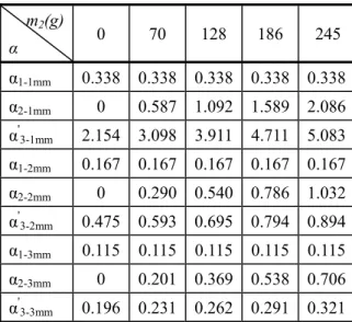
2 2 2 2 2 ) 2 ( 2 g Il Ml g Il l Ml I Ml g Il l Ml I Ml r G r G r G r G r G − + + ± + + = ⇒ω · · · ·(3-24) 2 2 2 2 2 2 ) 2 ( 2 g Il Ml g Il l Ml I Ml g Il l Ml I Ml r G r G r G r G r G − + + − + + = =ω α · · · (3-25) 2 2 2 2 2 2 ) 2 ( 2 g Il Ml g Il l Ml I Ml g Il l Ml I Ml r G r G r G r G r G − + + + + + = =ω β · · · (3-26) Putting π α 2 1= n f · · · ·(3-27) π β 2 2= n f · · · (3-28) where,

fn1: first frequency of the two-degree pendulum

fn2: second frequency of the two-degree pendulum

Subscrite n: thickness of the plate (1mm, 2mm and 3mm)

The angular positions of the two-degree pendulum were given as follows.

) sin cos )( 1 ( ) sin cos )( 1 ( 2 _{1 2} 2 _{3 4} 1 C t C t Mgl I t C t C Mgl I G G β β β α α α θ = − + + − + · · · ·· (3-29) ) sin cos ( ) sin cos ( 1 2 3 4 2 C αt C αt C βt C βt θ = + + + · · · ·(3-30) By the angular position of the two-degree pendulum, the motion of the two-degree pendulum could be solved. The solutions are useful to the lateral vibration.

3.3. Calculation of the center of gravity

the tow-degree pendulum motion. Fig. 3-2 shows the calculation model of the center of gravity of the plate beam h1 lG h2 l+h1+h2 dx _x m1g mg m2g A2 A1 A3

Figure.3-2 the calculation model of the center of gravity

Thus among the upper mass (m1), bottom mass (m2) and the beam mass (m), the following relation

was held. 0 ) 2 1 ( ) 2 1 ( ) 2 1 ( 1 1 2 1 2 1gl − h +mg l −h − l −m g l+h −l + h = m w w w · · · (3-31) where:

h1,h2: a length of upper and bottom load

l: length of the beam

lG: distance from the upper end to the center of gravity of the plate beam

Rearranging the above equation, the position of gravity center could be written as the following Equation.. ) ( 2 ) 2 ( ) 2 2 ( 2 1 2 2 2 1 2 1 m m m h m l m m h m m m lG _{+ +} + + + + + = · · · ·(3-32)

Table. 3-1. Calculated gravity center position under the experimental conditions

Bottom mass (g) 70 128 186 245

1mm(mm) 410.718 478.674 527.110 564.389

2mm(mm) 393.713 444.133 484.380 517.866 3mm(mm) 386.096 426.640 460.968 490.802

3.4. Calculation of inertia moment of force to the gravity center

Determining inertia moment of force to the gravity center of the plate beam is another important point in the calculation of the two-degree pendulous motion. To an arbitrary position, the inertia moment of force is given

dx Ax

dI _=ρ 2 _{· · · ·(3-33)}

Thus the calculated second moment of force of inertia to the gravity center is given as follows.

∫

∫

∫

+ + − − + − + + − − − + + = G G G l h h l l h l l h l h l l h l dx x A dx x A dx x A I 2 1 1 1 2 3 2 2 2 1 ρ ρ ρ G G G 1 1 · · · ·(3-34) Rearranging the upper equation, we obtain:

) ) ( ) (( 3 1 ) ) ( ) (( 3 1 ) ) ( ) (( 3 1 3 1 3 2 1 3 3 1 3 1 2 3 3 1 1 G G G G G G l h l l h h l A l h l h l A l l h A I − + − − + + + − − − + + − − − = ρ ρ ρ · · · (3-35) where,

A1, A2, and A3: area of cross-section of the upper load, the beam and the bottom load, respectively.

ρ: mass density

Table.3-2. calculated second moment of forces of inertia to the gravity center under the experimental conditions

Bottom mass (g) 70 128 186 245

1mm(_kg∗m2) _{0.0170 0.0225 0.0265 0.0298} 2mm(_kg∗m2) _{0.0217 0.0282 0.0335 0.0381} 3mm(_kg∗m2) _{0.0262 0.0333 0.0395 0.0451}

By the frequency equation of the two-degree pendulum, the frequency of the two-degree pendulum was determined under the experimental conditions. The results are shown in following tables in the case the different rope lengths and the different thicknesses of the plate beam.The following tables show the calculated results of the two-degree pendulum.

Table.3-3. First frequency of the two-degree pendulum as lr=170mm

Bottom mass (g) 70 128 186 245

1mm f11(Hz) 0.587 0.565 0.553 0.544

2mm f21(Hz) 0.603 0.582 0.568 0.558

3mm f31(Hz) 0.6104 0.591 0.577 0.567

Table 3-3 shows the first frequency of the two-degree pendulum decreases because the center of gravity of the plate beam decreases as the bottom load increases.

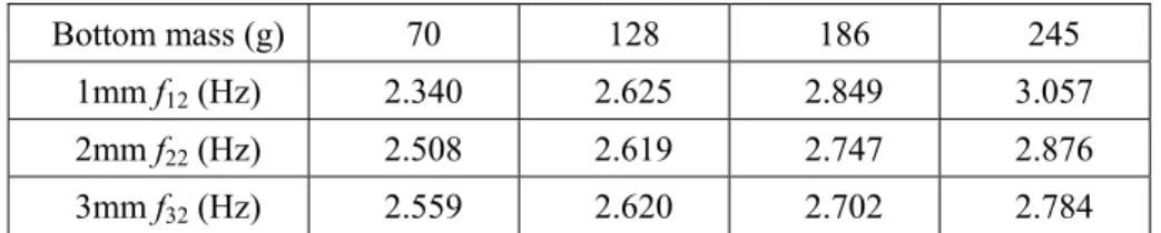
Table 3-4. Second frequency of the two-degree pendulum as lr=170mm

Bottom mass (g) 70 128 186 245

1mm f12(Hz) 2.340 2.625 2.849 3.057

2mm f22(Hz) 2.508 2.619 2.747 2.876

3mm f32(Hz) 2.559 2.620 2.702 2.784

Table 3-4 shows the second frequency of the two-degree pendulum increases because the center of gravity of the plate beam decreases and the inertia moment of force to the gravity center of the plate beam increases as the bottom load increases.

Table 3-5 shows the first frequencies of the two-degree pendulum decreases that caused by the center of gravity of the plate beam decrease as the bottom loads increase.

Table 3-6 shows the second frequency of the two-degree pendulum increase that caused by the center of gravity of the plate beam decrease and the inertia moment of force to the gravity center of the plate beam increase as the bottom loads increase.

The table 3-3, 3-5 and 3-4, 3-6 show the frequencies of the two-degree pendulum decreases as the hanging rope length increases. The first frequency of the two-degree pendulum decreases and the second frequency of the two-degree pendulum increases as the bottom load increases. The reason is the center of gravity of the pendulous vibration system decreases as the hanging rope length increases.

Table.3-5. First frequency of the two-degree pendulum as lr=120mm

Bottom mass (g) 70 128 186 245

1mm f11(Hz) 0.604 0.581 0.568 0.559

2mm f21(Hz) 0.622 0.599 0.584 0.573

3mm f31(Hz) 0.630 0.608 0.594 0.582

Table.3-6. Second frequency of the two-degree pendulum as lr=120mm

Bottom mass (g) 70 128 186 245

1mm f12(Hz) 2.777 3.041 3.301 3.544

2mm f22(Hz) 2.896 3.029 3.180 3.331

3mm f32(Hz) 2.952 3.028 3.125 3.227

3.6 Conclusion

Although the frequency of the two-degree pendulum was calculated by the above analysis, the vibration of the two-degree pendulum is not our researching object. While dealing with the lateral vibration, if both the lateral vibration and the vibration of the two-degree pendulum were considered together, theoretical analysis would became too complicated to be applied to a designing calculation of a practical vibroflot. The frequency of the two-degree pendulum was calculated to get important reference date in the designing calculation of a practical vibroflot.

3.7.References

(1). 吉川, ほか二人, 機械の力学, コロナ社, ISBN4-339-04273-0 (2). Mechanical Vibration Analysis and Computation, D.E. Newland. (3). L. Meirovitch: Analytical Methods in Vibration.

(4). D. J. Inman: Engineering Vibration

Chapter 4

Analysis and Experiment of Free Vibration

(Based on a Rectangular Working Model)

4.1 Introduction

In chapter 3, the analysis of the two-degree pendulous vibration was done basing on a rectangular beam. In this chapter, a theoretical analysis model of the free lateral vibration based on the rectangular working model was given and experimentally proved.

4.2. Analytical Method

In order to analyze the bending motion of the hanging beam, the coordinate was built as shown in Fig.4-1. The origin of the fixed coordinate X-O-Y was chosen at the top of the rope, the gravity direction was treated as X and the perpendicular direction to the gravity direction was treated as Y. Since the motion of the beam was a flexural vibration by the bending and pendulous vibration, the origin of the moving coordinate x-o-y was chosen at the top of the beam in the pendulous vibration, the axial direction of the beam was treated as x and the perpendicular direction to the beam axis was treated as y. The elastic vibration was treated in the moving coordinate system. The Lagrange equation was taken here.

where, 0 ) ( = ∂ ∂ − ∂ ∂ ∂ ∂ i i L L t θ& θ or ( ) ∂ =0 ∂ − ∂ ∂ ∂ ∂ y L y L t & · · · ·(4-1)

where, θi (i=1,2) stand for the swing angle of the rope and the beam in the pendulous vibration, y

stands for the displacement of the elastic of the beam in the moving coordinate system. And L is given as follows

U T

L= − · · · (4-2) where, T is the kinetic energy of the system, and U is the potential energy of the system. Here the mass of the rope was neglected for it is very small compared to the beam, so the energy of the system is only due to the beam. So any position on the beam in the fixed coordinate was given as follows;

y x ο X O Y 2 θ θ1 y x m m 1 2 m m 1 2 m g₀ '

Fig.1(a) Fig.1(b) Fig.1(c)

y x ο X O Y 2 θ θ1 m m 1 2 ο θ X Y G G r θ

Fig.1: Coordinate system of a suspended beam (a) Total view of the bending beam and the pendulous motion.

(b) Pendulous motion of the suspended rigid beam. (c) Bending motion of the suspended beam.

X-O-Y: world coordinate system.

x-o-y: local coordinate system on the suspended beam which is connected to the world coordinate

system though a suspending wire.

θ１:deflection angle of the rope.

θ２:deflection angle of the beam in a rigid motion.

∆θ:change in θ１due to an elastic motion of the beam m1, m2: top and bottom mass

XG, YG: position of the center of mass

Γ’, Γ:tension with and without elastic motion.

⎜⎜ ⎝ ⎛ + + = − + = 2 2 1 2 2 1 cos sin sin sin cos cos θ θ θ θ θ θ y x l Y y x l X r r _{· · · ·(4-3, 4)}

where, lr is the length of the rope.

⎜ ⎜ ⎝ ⎛ − + + = − − − − = 2 2 2 2 2 1 1 2 2 2 2 2 1 1 sin cos cos cos cos sin sin sin θ θ θ θ θ θ θ θ θ θ θ θ θ θ & & & & & & & & & & y y x l Y y y x l X r r _{· · · (4-5, 6)}

The kinetic energy T of the system is

dm Y X K m

∫

+ = 0 2 2 ₎ ( 2 1 _{& & · · · (4-7)}

where, m and dm are the total and elemental mass of the beam. And (_{X& +}2 _Y&2_{) is written as follows;}

) cos( 2 ) sin( 2 ) cos( 2 2 2 1 1 2 1 1 2 2 1 1 2 2 2 2 2 2 2 2 2 2 1 2 2 2 θ θ θ θ θ θ θ θ θ θ θ θ θ θ θ − + − + − + + + + + = + & & & & & & & & & & & & & & y l y l x l y x y y x l Y X r r r r · · · (4-8)

The potential energy U of the system is written as follows

dx x y EJ dm y x l g U l m r 2 0 2 2 2 2 1 0 ) ( 2 1 } sin ) cos 1 ( ) cos 1 ( {

∫

∫

∂ ∂ + + − + − = θ θ θ · · · (4-9)

where, E, J and g denote, respectively, modulus of elasticity, the second moment of force of area of the beam and the gravity acceleration.

Thus Eq.(4-2) was rewritten as follows

dx x y EJ dm y x l g dm Y X L l m r m 2 0 2 2 2 2 1 0 0 2 2 ) ( 2 1 } sin ) cos 1 ( ) cos 1 ( { ) ( 2 1

∫

∫

∫

∂ ∂ − + − + − − + = & & θ θ θ · · · ·(4-2')

Substituting Eq. (4-2') into Eqs. (4-1), we obtain the following equations

0 cos sin ) cos sin ( } sin sin cos { 0 0 2 0 2 2 2 2 2 1 2 1 0 = + − + − − + +

∫

∫

∫

rm m r m r r r G r G r dm y dm y ydm l g l l m && & & & && & && && θ θ θ θ θ θ θ θ θ θ θ θ θ · · · ·(4-10) 0 ) ) ( sin 2 cos sin cos ( ) sin sin cos ( ) ( 1 2 0 2 1 1 2 2 1 2 1 0 2 2 0 = − + − + + − + + + + +

∫

gy l y l y yy l y x l ydm l l gl l l m I l m G r r m r r r r r G r G r G r G G && & & & & & && & && && θ θ θ θ θ θ θ θ θ θ θ θ θ θ · · · (4-11) 0 ) ( ) sin sin cos ( 0 2 4 4 0 2 2 2 2 1 1 2 0 _∂ + = ∂ + ∂ ∂ + + − + _{r r r r}

_∫

m

_∫

l G y dx x y EJ dm t y g l l l

m θ&& θ&& θ θ& θ θ θ& ·· · · (4-12) When considering only the pendulous motion, Eqs.(4-10) and (4-11) were written as the following equations 0 = + + θ θ θ l g l && && · · · (4-13)

0 ) ( 2 _{2 0 1 0 2} 0 + + = +ml θ mll θ ml gθ I_{G G} && _rG && _G · · · ·(4-14) Eq.(4-13) and (4-14) are the fundamental Equation.s of the pendulous motion. From Eq.(4-14)-Eq.(4-13)×lG, 0 ) ( 2 1 0 2+ θ −θ = θ G G ml I && · · · (4-15) was obtained.

Eq. (4-15) shows the relationship between the moment of force of force and the relative angle (θ2-θ1)

around the center of gravity of the beam

Also from Newtown laws, the relationship between the relative angle (θr=θ2-θ1) and the tension Γ of

the rope around the center of gravity of the beam was written as follows: 0

sin

2+ΓG r =

G l

I θ&& θ · · · (4-16) where, Γ is the tension of the rope when only the pendulous motion was considered.

In the case θ2-θ1 is very small, sin(θ2-θ1) should be approximated as θ2-θ1, and then Eq.( 4-16) and

Eq.(4-15) should be same, so that the tension Γ was approxmated as follows,

g mo =

Γ · · · ·· · · (4-17) Furthermore, In the case that bending and pendulous motion were considered together, from Eq.( 4-11)-Eq.( 4-10)×lG, the following relationship was obtained.

0

2+Γl +∆M =

IGθ&& Gθr · · · ·· · · (4-18)

Where, △M was defined as follows

dm y y y l x y l l g M G G r r m ] 2 ) ( )} ( cos cos [{ 2 2 2 2 1 0 2 & & && & & θ θ θ θ θ + − + + + = ∆

_∫

· · · (4-19)

So the tension Γ was expressed in the case the bending and pendulous motion were considered together as follows, dm y y l l y l l l l l g m r G r r G r r m G r G r } sin ) cos ( ) cos {( ) sin cos ( 1 2 1 2 0 2 2 2 2 1 1 0 θ θ θ θ θ θ θ θ θ θ θ θ && & & & && && & && & + − + − + + + + = Γ

∫

· · · (4-20)