Spectral properties of weighted line digraphs (Designs, Codes, Graphs and Related Areas)

(1)

Spectral

properties of

weighted line digraphs

Etsuo Segawa,1 $*$

1 _{Graduate School of Information Sciences, Tohoku University}

Aoba, Sendai 980-8579, Japan

Abstract. In this paper, wetreat someweighted line digraphs which are induced by a connected

and undirected graph. For agiven graph$G$, the adjacencymatrixofthe weightedline digraph$W$ is

determined byaboundary operator from an arc-based spaceto a vertex-based space. Wesee that

dependingonthe boundary operator and the Hilbert spaces, $W$has diﬀerentkindofanunderlying

stochastic transition operator. As an application, we obtain the spectrum of the positive support

of cube ofthe Grover matrix ina large girthofthe graph.

1 Introduction

Quantum walk

was

proposed

as

iterations of aunitary operator

on

some

discrete space [10, 11]. Quantum walks (QWs) have been intensively studied since its eﬃciency of spatial

quantum search were shown i.g., [1] and see its reference for more detail. Now QWs are

investigated from various fields, for example, implementation in experiments, condensed

matter physics, probability theories, and graph theories and so on.

For agiven graph$G$, the spectralmappingtheorem ofquantumwalks have beenfounded

by Szegedy [2]. In this paper, we consider this spectral map to three kinds of quantum walks. First we consider a special classofquantum walks, which

can

be constructed

on

any (undirected) graphs and its spectrum has a relation to a random walk. This class of QW is called the Szegedy walk including the Grover walk. We refine the original one to

see

a

relation to a graph laplacian and the Grover walks which work well in the spacial quantum search for hypercube, Johnson graph and finite $d$-dimensional lattice and soon, see [1] and

its reference. The original Szegedy walk introduced by [2] is equivalent to square of the Szegedy walk treated here.

Secondly wetreat a quantum graph walk introduced by [8]. Recently, arelationship

be-tweenthisquantumwalkand thequantumgraph [4], which is asystemofalinearSchr\"odinger

equations with boundary conditions. has been found [8, 12]. In this paper, we develop this

study by connecting the spectrum of the original quantum graph and this quantum walk.

To this end, we apply the spectral map.

Finallywe also consider the cube ofpositive supportof the Groverwalk. There are some

trials to apply QW to graph isomorphism problems. For a matrix $M$_, the positive support

*email address [email protected]

Key words and phrases. Spectral mappingtheorem, Szegedywalk, Quantum graph, Positivesupportof

(2)

of$M,$ $M^{+}$, is denoted by

$(M^{+})_{i,j}=\{\begin{array}{l}1 :(M)_{i,j}\neq 00 : otherwise\end{array}$

It is suggested that the spectra of $(U^{3})^{+}$, which is the positive support of the cube of the Grover matrix $U^{3}$, outperforms distinguishing strongly regular graphs in [3].

Thispaper isorganized

as

follows. InSection2,weconstruct quantum walks

on

$\ell^{2}(m_{A}, A)$,

where$A$ is the set of thesymmetric arcsand

$m_{A}$ is apositive realvalued

measure.

In Section

3, first, we present the spectral mapping theorem from $C^{0}(G)$ to $C^{1}(G)$, which is the key in

ourpaper. secondly, we take three examples Szegedy walk [5, 2], quantum graphwalk [4, 8]

and the positive supports of the Grover walks [3, 6, 7] as applications.

2

Szegedy

walk:

reconsideration

Let $G=(V(G), E(G))$ be a connected and locally finite graph, where $V(G)$ _is _{the set of}

vertices and $E(G)$ _{is the set of all edges. We set} $A(G)=\{(u, v) : \{u, v\}\in E(G)\}$ asthe set

ofall arcs of$G$, and the origin vertex and terminal one of_{$e=(u, v)\in A(G)$} are denoted _by

$o(e)=u$ and $t(e)=v$. The inverse arc $e=(u, v)$ _are denoted by $\overline{e}=(v, u)$. We take

$C^{0}(G)=\{f:Varrow \mathbb{C}\}, C^{1}(G)=\{\psi : Aarrow \mathbb{C}\}$

as the space of allfunctionson$V(G)$ and$A(G)$, respectively. We preparepositivereal valued functions $m_{A}$ : $C^{1}(G)arrow C^{1}(G)$ and $m_{V}$ : $C^{0}(G)arrow C^{0}(G)$. For given such $m_{V}$ and $m_{A},$

we also set $\ell^{2}(m_{V};V)$ and $\ell^{2}(m_{A};A)$ as the square-summable functions with respect to the

inner product

$\langle f_{1}, f_{2}\rangle_{m_{V},V}=\sum_{u\in V(G)}\overline{f_{1}(u)}f_{2}(u)m_{V}(u)$, (2.1)

$\langle\psi_{1}, \psi_{2}\rangle_{m_{A},A}=\sum_{e\in A(G)}\overline{\psi_{1}(u)}\psi_{2}(e)m_{A}(e)$, (2.2)

respectively. Fromnowon, weconstruct the time evolution of aquantumwalkon $\ell^{2}(m_{A};A)$.

We set a complex valued function $w$ : $C^{1}(G)arrow C^{1}(G)$ to define boundary _operator $d$ :

$C^{1}(G)arrow C^{0}(G)$:

$(d \psi)(u)=\sum_{e:t(e)=u}\overline{w(\overline{e})}\psi(e)$. (2.3)

This operator takes just terminus one to get a unitary operator on $\ell^{2}(m_{A}, A)$, which is

dif-ferent from a “usual boundary operator. We introduce coboundary operator $d^{*}$ : _{$C^{0}(G)arrow$}

$C^{1}(G)$ satisfying $\langle d^{*}f,$$\psi\rangle_{mA}A,=\langle f,$$d\psi\rangle_{m_{V},V}$:

$\langle f, d\psi\rangle_{m_{V},V}=\sum_{u\in V}\overline{f(u)}\sum_{e:t(e)=u}\psi(e)\overline{w(\overline{e})}m_{V}(u)$

$= \sum_{e\in A}\psi(e)\overline{f(t(e))}\frac{m_{V}(t(e))\overline{w(\overline{e})}}{m_{A}(e)}m_{A}(e)$

(3)

So we have

$(d^{*}f)(e)=f(t(e)) \frac{m_{V}(t(e))w(\overline{e})}{m_{A}(e)}$. (2.4)

Put $S:C^{1}(G)arrow C^{1}(G)$ by $(S\psi)(e)=\psi(\overline{e})$. We define $U:C^{1}(G)arrow C^{1}(G)$ as follows.

$U=S(2d^{*}d-1_{A})$. (2.5)

Definition 1. $($Szegedy $walk on G(V, E)$)

When $U$

defined

in Eq. (2.5) is

norm

conservative in$\ell^{2}(A;m_{A})$ i. e., $||U\psi||_{m_{A},A}=||\psi||_{mA}A,$

for

any$\psi\in\ell^{2}(m_{A};A)$,

we

define

the quantum walk

as

follows:

The quantum walk witha unit

initial state $\psi_{0}\in\ell^{2}(m_{A};A)$ is

defined

by the following sequence

of

probability distributions

$\{\mu_{n}^{(\psi 0)}\}_{n\in N}$, where $\mu_{n}^{(\psi_{0})}$

: $Aarrow[O$_,1$]$ is $deter\gamma nined$ by

$\mu_{n}^{(\psi 0)}(e)=|\psi_{n}(e)|^{2}m_{A}(e)$. (2.6)

Here $\psi_{n}$ is the n-th iteration

of

$U$ i.e., $\psi_{n}=U\psi_{n-1}(n\geq 1)$_. In particular,

we

define

the finding probability

_of

a quantum walker at time $n$ in location

of

$u\in V,$ $\nu_{n}:Varrow[O$, 1$]$, by

$\nu_{n}^{(\psi_{0})}(u)=\sum_{e:t(e)=u}\mu_{n}^{(\psi_{0})}(e)$.

We provide two ways which give the operator $U$ definedin Eq. (2.5) preserving the

norm

withrespect to $\rangle_{mA}A,\cdot$ Both of them have some underlying dynamics on $C^{0}(G)$; thefirst

one is a random walk while the second one is a laplacian. (1) Setting 1

(a) $\sum_{e:o(e)=u}|w(e)|^{2}=1$ for all $u\in V$;

(b) $m_{V}(u)=1,$ $m_{A}(e)=1$ for all $u\in V$ _and $e\in A.$

(2) Setting 2

(a) $\sum_{e:o(e)=u}w(e)=1$ for all $u\in V$;

(b) $m_{A}(e)=m_{V}(o(e))w(e)=m_{V}(t(e))w(\overline{e})$ for all $e\in A.$

We call thecondition (2) in Setting 2 “extended detailedbalanced condition”’ Wecaneasily check that both of the coboundary operators $d^{*}$ in the setting of(1) and (2) are isometric.

Proposition 1. Both settings (1) and (2) imply that $U$ preserves the norm.

Proof.

It is easy to check that both settings (1) and (2) provide

$\langle S\psi_{1}, S\psi_{2}\rangle_{mA}A,=\langle\psi_{1}, \psi_{2}\rangle_{m_{A},A}$. (2.7)

$dd^{*}=1_{V}$ (2.8)

By Eq. (2.7), it holdsthat

$\langle U\psi,$$U\psi\rangle_{m_{A},A}=\langle S(2d^{*}d-1_{A})\psi,$$S(2d^{*}d-1_{A})\psi\rangle_{mA}A,=\langle(2d^{*}d-1_{A})\psi,$ $(2d^{*}d-1_{A})\psi\rangle_{m_{A},A}$

(4)

bom Eq. (2.8), the inner product of the first term of RHS is rewritten by

$\langle d^{*}d\psi, d^{*}d\psi\rangle_{m_{A},A}=\langle d\psi, d\psi\rangle_{m_{V},V}$

$=\langle\psi, d^{*}d\psi\rangle_{m_{V},V}=\langle d^{*}d\psi, \psi\rangle_{m_{V},V}$. (2.10)

Inserting Eqs. (2.10) into (2.9), wehave $||U\psi||_{m_{A},A}^{2}=||\psi||_{m_{A},A}^{2}.$ $\square$

We take $U_{1}$ and $U_{2}$ as the time evolution of quantum walks with respect to the inner

products under the settings of 1 and 2, respectively. Equivalently, $U_{1}$ and $U_{2}$ are expressed

by

$(U_{1} \psi)(e)=\sum_{f:o(e)=t(f)}(2w_{1}(e)\overline{w_{1}(\overline{f})}-\delta_{e,\overline{f}})\psi(f)$, (2.11)

$(U_{2} \psi)(e)=\sum_{f:o(e)=t(f)}(2w_{2}(\overline{f})-\delta_{e,\overline{f}})\psi(f)$, (2.12)

where

$(d_{j} \psi)(u)=\sum_{e:t(e)=u}\psi(e)\overline{w_{j}(\overline{e})}(j=1,2)$ (2.13)

$(d_{j}^{*}f)(e)=\{\begin{array}{ll}f(t(e))w_{1}(\overline{e}) :j=1,f(t(e)) :j=2.\end{array}$ (2.14)

Here $w_{j}$ : $Aarrow \mathbb{C}(j=1,2)$ satisfy settings 1 (a) and 2, respectively. These two quantum

walks are essentially the same in the following meaning:

Proposition 2. Assume that $w_{1}^{2}(e)=w_{2}(e)>0(e\in A)$. For$\psi\in C^{1}(G)$, let $\psi_{n}^{(\psi)}=U_{1}^{n}\psi,$

$\tilde{\psi}_{n}^{(\psi)}=U_{2}^{n}\psi$ and $\mu_{n}^{(\psi)}$

and $\tilde{\mu}_{n}^{(\psi)}$

be the distributions

_of

$QWs$ at time $n$

defined

in Eq. (2.6)

under the settings 1 and 2, respectively. Then we have (1) $\tilde{\psi}_{n}(\psi_{0})_{=\mathfrak{D}^{-1/\psi 0)}}2\psi_{n}^{(\mathfrak{D}^{1/2}}$

(2) $\tilde{\mu}_{n}^{(\psi_{0})}=\mu_{n}^{(\psi_{0})}\mathfrak{D}^{1/2}$

Proof.

For the proofofpart 1, comparing Eq. (2.11) with Eq. (2.12) immediately provides that if$w_{1}^{2}(e)=w_{2}(e)\in \mathbb{R}$, then we have

$U_{2}=\mathfrak{D}^{-1/2}U_{1}\mathfrak{D}^{1/2}$, (2.15)

where $(\mathfrak{D}\psi)(e)=m_{A}(e)\psi(e)$. Equation (2.15) implies part 1. For the _proof_of_part _{2, using}

Eq. (2.15),

$\tilde{\mu}_{n}^{(\psi 0)}(e)=|\tilde{\psi}_{n}(e)|^{2}m_{D}(e)=|\mathfrak{D}^{1/2}(\mathfrak{D}^{-1/2}U_{1}^{n}\mathfrak{D}^{1/2}\psi_{0})(e)|^{2}=|(U_{1}^{n}\mathfrak{D}^{1/2}\psi_{0})(e)|$

$=\mu_{n}^{(\mathfrak{D}^{1/2}}\psi_{0)}(e)$

(5)

3 Spectral

map

3.1 Spectral map

For a given boundary operator $d$, let us define an operator on $C^{1}(G)$ by

$W=S(cd^{*}d-1_{A})$, (3.16)

We assume that the following value $c’$ is constant with respect to the vertices ofthe given

graph:

$c’= \sum_{e:t(e)=u}\frac{m_{V}(t(e))|w(\overline{e})|^{2}}{m_{A}(e)}$ for anyu $\in V.$

This assumption implies $dd^{*}=1_{V}$. We also

assume

$cc’\neq 1$ for

some

technical

reason.

Remark that in the present stage, $W$ has no restriction of the norm conservation. We

provide examples by taking appropriate functions $m_{A},$ $m_{V},$ $w$ and parameter $c\in \mathbb{C}$ in the

later subsection. We set

$\mathcal{H}_{\pm}=\{\psi\in\ell^{2}(A):\psi(\overline{e})=\pm\psi(e)(e\in A$

The following lemmais the key in this paper, which is an extended version of Proposition 1

in [5].

Lemma 1. Let$G$ be a

finite

graph. Put _{$\varphi(x)=(x+(cc’-1)x^{-1})/c$} and$\mathcal{L}=d^{*}(C^{1}(G))+$

$Sd^{*}(C^{1}(G))\subseteq C^{1}(G)$. Then we have $W(\mathcal{L})=\mathcal{L}$ and

$\sigma(W|_{\mathcal{L}})=\{\begin{array}{ll}\varphi^{-1}(\sigma(d^{*}Sd)\backslash \{\pm c’\})U\{\pm(cc’-1)\} :\pm c’\in\sigma(dSd^{*})\varphi^{-1}(\sigma(d^{*}Sd)\backslash \{c’\})\cup\{cc’-1\} :c’\in\sigma(dSd^{*})\varphi^{-1}(\sigma(d^{*}Sd)\backslash \{-c’\})\cup\{-(cc’-1)\} :-c’\in\sigma(dSd^{*})\varphi^{-1}(\sigma(d^{*}Sd)) :otherwise\end{array}$ (3.17)

$\sigma(W|_{\mathcal{L}^{\perp}})=\{\begin{array}{ll}\{1, -1\} :\mathcal{H}_{-}\cap ker(d)\neq\{0\}, \mathcal{H}_{+}\cap ker(d)\neq\{0\}\{1\} :\mathcal{H}_{-}\cap ker(d)\neq\{0\}, \mathcal{H}_{+}\cap ker(d)=\{0\}\{-1\} :\mathcal{H}_{-}\cap ker(d)=\{0\}, \mathcal{H}_{+}\cap ker(d)\neq\{0\}\emptyset :otherwise.\end{array}$ (3.18)

The eigenfunction

_for

$\lambda\in\sigma(W|_{\mathcal{L}})$, $\psi_{\lambda}\in C^{1}(G)$, can be expressedby using the eigenfunction

of

$dSd^{*}for$ $\varphi(\lambda)\in\sigma(dSd^{*})$, $f_{\varphi(\lambda)}\in C^{0}(G)$, as

follows:

$\psi_{\lambda}=\{\begin{array}{ll}(d^{*}-\lambda Sd^{*})f_{\varphi(\lambda)} :\lambda\neq\{\pm(cc’-1)\}\pm d^{*}f_{\varphi(\lambda)} :\pm c’\in\sigma(dSd^{*}) , \lambda\in\{\pm(cc’-1)\}\end{array}$ (3.19)

Proof.

From the properties of$d$ and $S$, it holds that for any $n\in \mathbb{N},$

$[Wd^{*} WSd^{*}]=[d^{*} Sd^{*}]\tilde{T}$. _(3.20) Herewe put

(6)

By multiplying arbitrary $T[f_{1}, f_{2}]$ to both sides of Eq. (3.20), we have $W(\mathcal{L})\subset \mathcal{L}$. For any $h\in \mathcal{L}$, there exist $f,$$9\in C^{0}(G)$ such that $h=d^{*}f+Sd^{*}g$. By Eq. (3.20)

$W(d^{*}(c(dSd^{*})f+g)-Sd^{*}f)=(cc’-1)h,$

whichimplies $W(\mathcal{L})\supset \mathcal{L}$ since $cc’\neq 1$. Thus $W(\mathcal{L})=\mathcal{L}$. Fhrom now on, we choose a pair of

nonzero functions $(f, g)\in C^{0}(G)\cross C^{0}(G)$ sothat

$\tilde{T}\{\begin{array}{l}fg\end{array}\}=\lambda\{\begin{array}{l}fg\end{array}\}$

.

(3.21)

Eq. (3.21) is equivalent to

$g=-\lambda f$ (3.22)

$(\varphi(\lambda)-dSd^{*})f=0$ (3.23)

From Eqs. (3.21) and (3.22), wehave

$W(1_{A}-\lambda S)d^{*}f=\lambda(1_{A}-\lambda S)d^{*}f$ (3.24)

By the way, let $v\in \mathbb{R}$ and _{$f\in C^{0}$} be an eigenvalue and its eigenfunction $dSd^{*}$, which is a

self adjoint operator. Set $\Pi=(1/c’)d^{*}d.$ $\Pi$is aprojection onto _{$d^{*}(C^{0}(G))$}. Taking _{$d^{*}f=\psi,$}

we have

$|v|^{2}||f||^{2}=||dSd^{*}f||^{2}=||d\Pi S\Pi\psi||^{2}=c’||\Pi S\Pi\psi||^{2}\leq c’||\Pi\psi||^{2}=(c’)^{2}||f||^{2}.$

Thus $\nu\leq c’$. The fourth equality holds if and only if_{$Sd^{*}f=d^{*}f$} or _{$Sd^{*}f=-d^{*}f$}_, _which

implies that

$\nu=\pm c’$_if _and_only _if$d^{*}f\in \mathcal{H}_{\pm}$

Now from Eq. (3.24), we consider the following two cases.

(1) $(1_{A}-\lambda S)d^{*}f=0$ case. From the above observation, this situation is equivalent to

(

$\lambda=1$ and $c’\in\sigma(T)$” or $\lambda=-1$ _and $-c’\in\sigma(T)$”, and $f\in ker(dSd^{*}\pm c$

Remark that $Wd^{*}f=\pm(cc’-1)d^{*}f$ and $\varphi^{-1}(\pm c’)=\{\pm 1,$$\pm(cc’-1$ So we _{have if}

$\pm c’\in\sigma(dSd^{*})$, then $\pm(cc’-1)\in\varphi^{-1}(\pm c’)\backslash \{\pm 1\}\subset\sigma(W|_{\mathcal{L}})$.

(2) $(1_{A}-\lambda S)d^{*}f\neq 0$ case. This situation implies $\lambda\in\sigma(U)$. Equation (3.23) implies that $\lambda\in\varphi^{-1}(\sigma(d^{*}Sd)\backslash \{\pm c’\})$. (3.25)

In this case, the eigenfunction $(1_{A}-\lambda S)d^{*}f\not\in \mathcal{H}_{\pm}$ but $(1_{A}-\lambda S)d^{*}f\in \mathcal{H}_{+}+\mathcal{H}_{-}.$

$\dim(\mathcal{H}_{+}\cap L)=|V|$ Combining

cases

(1) and (2), we have Eq. (3.17) and Eq. (3.19).

In the following, we show Eq. (3.18). Since $\mathcal{L}^{\perp}=ker(d)\cap ker(dS)$, we have

$W(\psi+S\psi)=-(\psi+S\psi)\in \mathcal{H}$_-and $W(\psi-S\psi)=\psi+S\psi\in \mathcal{H}_{+}$. (3.26)

We set $c_{\pm}=\mathcal{L}^{\perp}\cap \mathcal{H}_{\mp}$. We have

$W\psi\pm=\pm\psi\pm$, for any $\psi_{\pm}\in c_{\pm}$. (3.27)

For $\psi\in \mathcal{H}_{\mp}\cap ker(d)$, _{$dS\psi=\pm d\psi=0$}holds which implies $\mathcal{H}_{\mp}\cap ker(d)=c_{\pm}$. It is completed

(7)

3.2 Example 1: Szegedy

walk

We consider the spectral map of the Szegedy walk treated in Sect. 2. The parameter $c$ and

functions $m_{A},$ $m_{V}$ and $w$ are in the following table:

Let a selfadjoint operator on $C_{0}(G)$ be

$(Tf)(u)= \sum_{e:o(e)=u}w_{1}(e)\overline{w_{1}(\overline{e})}f(t(e))$

and a Laplacian operator be

$(Lf)(u)= \sum_{e:o(e)=u}w_{2}(e)f(t(e))-f(u)$.

Proposition 3. Put$\varphi_{1}(x)=(x+x^{-1})/2,$ $\varphi_{2}(x)=(x+x^{-1})/2-1.$

$\sigma(U_{1})=\{\begin{array}{ll}\varphi_{1}^{-1}(\sigma(T))\cup\{\pm 1\} :|E|-|V|+1_{\{1\in\sigma(T)\}}>0, |E|-|V|+1_{\{-1\in\sigma(T)\}}>0\varphi_{1}^{-1}(\sigma(T))\cup\{1\} :|E|-|V|+1_{\{1\in\sigma(T)\}}>0, |E|-|V|+1_{\{-1\in\sigma(T)\}}\leq 0\varphi_{1}^{-1}(\sigma(T))\cup\{-1\} :|E|-|V|+1_{\{1\in\sigma(T)\}}\leq 0, |E|-|V|+1_{\{-1\in\sigma(T)\}}>0\varphi_{1}^{-1}(\sigma(T)) : |E|-|V|+1_{\{1\in\sigma(T)\}}\leq 0, |E|-|V|+1_{\{-1\in\sigma(T)\}}\leq 0\end{array}$

(3.28)

$\sigma(U_{2})=\{\begin{array}{ll}\varphi_{2}^{-1}(\sigma(L)) : G is a tree\varphi_{2}^{-1}(\sigma(L))\cup\{1\} :G has just one cycle and not bipartite\varphi_{2}^{-1}(\sigma(L))\cup\{1\}\cup\{-1\} :otherwise\end{array}$ (3.29)

Proof.

By a simple observation, we can see that

$d_{1}^{*}Sd_{1}=T, d_{2}^{*}Sd_{2}=L+1_{V}$. (3.30)

We should remark that $L+1_{V}=\tau P$, where $P$ is a transition matrix of random walk:

$(Pf)(u)= \sum_{e:t(e)=u}w_{2}(e)f(e)$. In the setting of $U_{2}$, since $w_{2}$ is reversible, then $\sigma(^{T}P$) $=$

$\sigma(P)$ holds, which implies $\sigma(^{T}P$) $=\sigma(T)$ when $w_{2}=w_{1}^{2}.$ _$Rom$ the reversibility of the

stochastic process described by transition matrix $P$, it holds that _{$m_{1}=1$} and _{$m_{-1}=$}

$1_{\{Gisbipartite\}}$. From now on, we consider the dimensions of$c_{\pm}$

.

By Eq. (3.19) and $\varphi^{-1}(v)\in$

$\{\lambda, \overline{\lambda}\}$ with _{$v={\rm Re}(\lambda)$}, we observe

$\psi_{\lambda}+\lambda\psi_{\overline{\lambda}}\in\{\begin{array}{ll}\mathcal{H}_{-}\backslash \{0\} :\nu\neq-1\{0\} :\nu=-1\end{array}$

(8)

Therefore

$\dim(\mathcal{L}\cap \mathcal{H}_{+})=|V|-m_{-1}$ and$\dim(\mathcal{L}\cap \mathcal{H}_{-})=|V|-m_{1}$. (3.31)

Remarking$\dim(\mathcal{H}_{\pm})=|E|$, by Eq. (3.31),

$\dim(C_{+})=\dim(\mathcal{H}_{-})-\dim(\mathcal{L}\cap \mathcal{H}_{-})=|E|-|V|+m_{1}$ (3.32)

$\dim(C_{-})=\dim(\mathcal{H}_{+})-\dim(\mathcal{L}\cap \mathcal{H}_{+})=|E|-|V|+m_{-1}$ (3.33)

We should remark that

$|E|-|V|\{\begin{array}{ll}=-1 :G is a tree=0 :G has one cycle\geq 1 : G has at least 2 cycles\end{array}$ (3.34)

Combining Eqs. (3.32), (3.33) and Eq. (3.27) with Eq. (3.34) leads to Eq. (3.18).

Then Lemma 1 completesthe proof. $\square$

3.3 Example

2: Quantum graph walk

Quantum graph is asystem of linearSchr\"odiner equations on ametric graph with boundary conditions at each vertex. In the metric graph, each edge has a euclidean length, and there exists a one-dimensional plain wave on each edge. On $e\in A(G)$ whose euclidean length is

$L_{e}=L_{\overline{e}}$, we determine _{$x\in[0, L_{e}]$} as the distance from_$o(e)$. Theplainwave on

$e\in A(G)$ at

$x$ is described by using some complex numbers $a_{e},$$b_{e}$ as follows.

$\phi_{e}(x)=a_{e}e^{ikx}+b_{e}e^{-ikx}, (x\in[O, L_{e}])$ _(3.35)

Sincethe plain

wave

on each edge is independent of the arc direction, we should impose the following condition to $\phi_{e}.$

$\phi_{\overline{e}}(x)=\phi_{e}(L_{e}-x)e\in A(G)$ (3.36)

Combining Eqs. (3.35) and (3.36), $\phi_{e}(x)$ is rewritten by

$\phi_{e}(x)=a_{e}e^{ikx}+a_{\overline{e}}e^{ik(L-x)}$. _(3.37)

The boundary conditions at each vertex are as follows:

(1) For every $u\in V$ _and _for _all $e_{1}$, .

.

. ,$e_{\kappa}\in A(G)$ with $u=o(e_{1})=o(e_{2})$, there exists $\theta_{u}\in \mathbb{C}$ such that

$\phi_{e_{1}}(0)=\cdots=\phi_{e_{\kappa}}(0)=\theta_{u}.$

(2) For every$u\in V$_, there exists $\alpha_{u}\in[0, \infty]$ such that

(9)

Definition 2. Let $\psi_{n}\in C^{1}(G)(n\in \mathbb{N})$ be determined by the iterations

of

$\tilde{U}$ i.e., $\psi_{n}=$ $\tilde{U}\psi_{n-1}$, where $( \tilde{U}\psi)(e)=e^{ikL_{e}}\sum_{f:t(f)=o(e)}).$ Here $\tau_{u}=\frac{2}{\deg(u)+i\alpha_{u}/k}.$

The quantum graph walk is sequence

_of

distributions $\{\mu_{n}\}_{n\in N}$ obtained by $\mu_{n}(e)=|\psi_{n}(e)|^{2}.$

Note that $\tilde{U}$

is a unitary operator i.e., $\tilde{U}\tilde{U}^{*}=\tilde{U}^{*}\tilde{U}=1_{A}$.

Set $\psi\in C^{1}(G)$ with $\psi(e)=a_{e}.$

If $(a_{e})_{e\in A}$ satisfies the boundary conditions (1) and (2) with $\psi\neq 0$, then we say that the

quantum graph has non-trivial solution.

Proposition 4. [8] The quantum graph walk has a non-trivial solution

_if

and only

_if

$1\in$

$\sigma(\tilde{U})$.

Rom now on we restrict ourselves to consider the following simple case to make $\tilde{U}$ be able to apply the spectral map of Lemma 1.

Lemma 2.

_If

$L_{e}=L$

for

any $e\in A,$ $\deg(u)=\kappa$ and$\alpha_{u}=a$

for

any $u\in V$, then we have

$\tilde{U}=e^{ikL}S(cd^{*}d-1_{A})$_, _(3.38)

where

$c= \frac{2\kappa}{\kappa+iq(k)}, w(e)=\frac{1}{\sqrt{\kappa}}, m_{V}(u)=1, m_{A}(e)=1.$

Here we put$q(k)=\alpha/k.$

Remark that in this setting the boundary operator $d$ is given by

$(d \psi)(u)=\frac{1}{\sqrt{\kappa}}\sum_{e:t(e)=u}\psi(e)$.

We can easilycheck that $dd^{*}=1_{V}$ which implies$c’=1.$

Proposition 5. Let $P$ be a stochastic transition operator

of

the simple random walk on

$G(V, E)$. _Then _the _spectrum

_of

_the _{quantum graph} _{walk under the} _setting

_of

$L_{e}=L$

for

any

$e\in A,$ $\deg(u)=\kappa$ and $\alpha_{u}=\alpha$

for

any$u\in V$, we have

$e^{-ikL} \sigma(\tilde{U})=e^{i\arg(\tau)}\varphi_{1}^{-1}(\frac{\kappa}{\sqrt{\kappa^{2}+q^{2}(k)}}\sigma(P))$

$\{\emptyset\}$ : $G$ is a tree”’ or $q(k)\neq 0$ _and $G$ has at most one cycle

$\cup$ $\{$

{1}

: $tq(k)=0$ and$G$ hasjust one cycle whose length is odd (3.39)

(10)

Proof.

Eq. (3.23)implies

$\det(\lambda^{2}-cJ\lambda+c-1)=0$_, (3.40) where $J=dSd^{*}$ _{is expressed by}

$(Jf)(u)= \sum_{e:t(e)=u}\frac{1}{\sqrt{\deg(u)\deg(o(e))}}.$

Since $P$ is reversible, $\sigma(P)=\sigma(J)$ holds. Taking$\gamma=\arg(\tau)\in[\pi/2, \pi/2]$, we have

$c-1=e^{2i\gamma}$ _and $c=2e^{i\gamma}\cos\gamma$. (3.41)

Inserting Eq. (3.41) into Eq. (3.40) provides

$\det(\frac{(e^{-i\gamma}\lambda)-(e^{-i\gamma}\lambda)^{-1}}{2}-\frac{\kappa}{\sqrt{\kappa^{2}+q^{2}(k)}}P)=0.$

Weshould remark that since $1\in\sigma(P)$with simple multiplicity, then$1\in\kappa/\sqrt{\kappa^{2}+q^{2}(k)}\sigma(P)$

if and only if $q(k)=0$. and also remark that since $-1\in\sigma(P)$ if and only if$G$ is bipartite

and $q(k)=0$, then $-1\in\kappa/\sqrt{\kappa^{2}+q^{2}(k)}\sigma(P)$ if and only if_$q(k)=0$ and $G$is bipartite. Put

$M_{+}=|E|-|V|+1_{\{q(k)=0\}}$ and $M_{-}=|E|-|V|+1_{\{q(k)=0andGisbipartite\}}$. Let $b(G)$ be the

number of the essential cycles of$G$

.

So the following statement holds:

Thus we cancomplete the proofby applying the last half of the proof of Proposition 2. $\square$ Corollary 1. Set $A=\{k^{2}\in[0, \infty$) $:1 \in e^{i(kL+\arg(\tau))}\varphi_{1}^{-1}(\frac{\kappa}{\kappa+q^{2}(k)}\sigma(P))\}$

.

The spectrum

of

the quantum graph walk is expressed as

_follows:

$\{\begin{array}{ll}A : G is a treeA\cup\{(\frac{2n\pi}{L})^{2}:n\in \mathbb{N}\}\cup\{(\frac{(2n+1)\pi}{L})^{2}:n\in \mathbb{N}\} : G has at least one cycle\end{array}$

3.4 Example 3:

Positive

support of the

Grover

walk

Recently there are some trials to apply QW to graph isomorphism problems. For a matrix

$M$, thepositive support of$M,$ $M^{+}$, is denoted by

$(M^{+})_{i,j}=\{\begin{array}{l}1 :(M)_{i,j}\neq 00 :otherwise\end{array}$

It is suggested that the spectra of $(U^{3})^{+}$, which is the positive support of the cube of the

Grover matrix $U^{3}$, outperforms distinguishing strongly regular graphs in [3]. It

seems to be that not only the Grover matrix $U$ itself but the positive support $(U^{n})^{+}$ of its n-th power

is an important operator of a graph. For a first step, in this section, we consider $\sigma(U^{3})^{+}$

(11)

Proposition 6. [6] Let$G$ be a connected and$\kappa$-regular graph with$g(G)\geq 5$

.

Then

we

have

$(U^{3})^{+}=(U^{+})^{3}+^{T}U^{+}$_. _(3.42)

We can rewrite $U^{+}$ as follows:

Lemma 3. When we take $m_{A}(e)=1,$ $m_{V}(u)=1$ and $w(e)=1$, then we have

$U^{+}=S(d^{*}d-1_{A})$

The results on $(U)^{+}$ and $(U^{2})^{+}$ have already appeared in [6, 7]. In this paper, we newly

obtain $(U^{3})^{+}$

case

as follows.

Proposition 7. Assume that $G$ is a connected and $\kappa$-regular graph with $g(G)\geq 5$. Let $M$ be the adjacency matrix

_of

G. We set

$s_{\pm}^{(1)}(x)= \frac{x}{2}\pm\frac{\sqrt{x^{2}-4\kappa+4}}{2}$ , (3.43) $s_{\pm}^{(2)}(x)= \frac{x^{2}-2\kappa+4}{2}\pm\frac{x\sqrt{x^{2}-4\kappa+4}}{2}$ _(3.44) and $s_{\pm}^{(3)}(x)= \frac{x(x^{2}+4-3\kappa)}{2}$ $\pm\frac{1}{2}\sqrt{x^{6}+2(2-3\kappa)x^{4}+(13\kappa^{2}-24\kappa+16)x^{2}-8(\kappa-1)(\kappa^{2}-2\kappa+2)}$

.

_(3.45) Then we have $\sigma((U)^{+})=\{s_{\pm}^{(1)}(\lambda) : \lambda\in\sigma(M)\}\cup\{1\}^{|E|-|V|}\cup\{-1\}^{|E|-|V|}$ _(3.46) $\sigma((U^{2})^{+})=\{s_{\pm}^{(2)}(\lambda):\lambda\in\sigma(M)\}\cup\{2\}^{2(|E|-|V|)}$ _(3.47) $\sigma((U^{3})^{+})=\{s_{\pm}^{(3)}(\lambda) : \lambda\in\sigma(M)\}\cup\{2\}^{|E|-|V|}\cup\{-2\}^{|E|-|V|}$ _(3.48)

Proof.

The proofs ofcases of $(U)^{+}$ and $(U^{2})^{+}$ can be seen in [6, 7] So we provide only the

prooffor the $(U^{3})^{+}$ case. Since $\tau U^{+}=SU^{+}S$ _holds, _{by Eq.} _(3.20), _we _have

$[^{T}U^{+}d^{*} \tau U^{+}Sd^{*}]=S[U^{+}Sd^{*} U^{+}d^{*}]$

$=S[Sd^{*} d^{*}]\tilde{T}’$

$=[d^{*} Sd^{*}]\tilde{T}’$, _(3.49)

where

$\tilde{T}=\{\begin{array}{lll} 0 -1_{V}(k -1)1_{V} M\end{array}\}$ and $\tilde{T}’=\{\begin{array}{ll}0 1_{V}1_{V} 0\end{array}\}\tilde{T}\{\begin{array}{ll}0 1_{V}1_{V} 0\end{array}\}.$

Using Eq. (3.20) again,

(12)

Inserting Eqs. (3.49), (3.50) into Proposition (6) provides

$[(U^{3})^{+}d^{*} (U^{3})^{+}Sd^{*}]=[d^{*} Sd^{*}](\tilde{T}^{3}+\tilde{T}’)$ (3.51)

Now we consider the spectra of $\tilde{T}^{3}+\tilde{T}’$.

Since $M=M^{*},$ $M$ is decomposed by $M=$ $\sum_{\lambda\in\sigma(M)}\lambda\Pi_{\lambda}$, where $\Pi_{\lambda}$ is the orthogonalprojectiononto the eigenspaceofeigenvalue$\lambda$. By

Eq. (3.51),

$\tilde{T}^{3}+\tilde{T}’=\sum_{\lambda\in\sigma(M)}\Lambda(\lambda)\otimes\Pi_{\lambda}$. (3.52)

Here

$\Lambda(\lambda)=\{\begin{array}{lllll} -\lambda(\kappa-2) -\lambda^{2}+2\kappa -2(\kappa -\kappa -1)(\lambda^{2}+1)-1 \lambda(\lambda^{2} -2\kappa+2)\end{array}\}$

A simple computation gives

$\sigma(\Lambda(\lambda))=\{s_{\pm}^{(3)}(\lambda)\}.$

From the above, we obtain $2|V|$ eigenvalues of $(U^{3})^{+}$. All the $2|V|$ eigenvectors in $\mathcal{L}\equiv$ $d^{*}(C^{0}(G))+Sd^{*}(C^{0}(G))$ are

$\{(\lambda^{2}-2\kappa+2)d^{*}f_{\lambda}-(\lambda(\kappa-2)-s_{\pm}^{(3)}(\lambda))Sd^{*}f_{\lambda}$ : $\lambda\in\sigma(M)\}.$

Here $f_{\lambda}\in ker(\lambda-M)$. Note that since $(U^{3})^{+}$ is no longer ensured its regularity, there may

exist $\lambda\in\sigma(M)$ such that $s_{+}(\lambda)=s_{-}(\lambda)\equiv s(\lambda)$. In such a case, the geometric multiplicity

of$s(\lambda)$ is dimker$(T-\lambda)$ while the algebraic multiplicity is 2dimker(T–A).

Next weconsider the other invariantsubspace $\mathcal{L}^{\perp}$

. It holds that$\mathcal{L}^{\perp}=ker(d)\cap ker(dS)=$

$(ker(d)\cap \mathcal{H}_{+})\oplus(ker(dS)\cap \mathcal{H}_{+})$. For $\psi\in ker(d)\cap \mathcal{H}\pm$, we can check that $(U^{+})^{3}\psi=\mp 2\psi.$

Therefore the algebraic multiplicities ofeigenvalues $\pm 2$ are _$|E|-|V|.$ $\square$

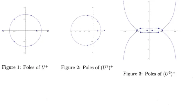
Let $Z_{G}^{(j)}(u)= \prod_{\lambda\in\sigma((U))}j+(1-u\lambda)^{-1},$ _{$(j\in\{1,2,3$} The following figure depict the _poles

of$Z_{G}^{(j)}(u)$ for the Petersen graph.

Figure 1: Poles of$U^{+}$ Figure 2: Poles of $(U^{2})^{+}$

(13)

Acknowledgment ES thanks to the financial supports of the Grant-in-Aid for Young

Sci-entists (B) and ofScientific Research (B) Japan Societyfor the Promotion ofScience (Grants No.25800088, No.23340027).

References

[1] A. Ambainis, Quantum walks and their algorithmic applications, Int. J. Quantum Inf. 1 (2003),

pp.507-518.

[2] M. Szegedy, Quantum speed-up of Markov chain based algorithms, Proc. 45th IEEE

Sympo-siumon Foundations of Computer Science (2004), pp.32-41.

[3] D. Emms, E. R. Hancock, S. Severini, R. C. Wilson, A matrix representationofgraphs and

its spectrumas agraph invariant, Electr. J. Combin. 13, R34 (2006).

[4] P. Exner, P. Seba, Freequantum motion on a branching graph, Rep. Math. Phys. 28 (1989),

pp.7-26.

[5] Yu. Higuchi, N. Konno, I. Satoand E. Segawa, Spectral and asymptotic propertiesof Grover

walks on crystal lattices, Journalof Functional Analysis 267 (2014), pp.4197-4235.

[6] Yu. Higuchi, N. Konno, I. Sato,E. Segawa, A noteonthediscrete-time evolutions ofquantum

walkon a graph, Journal of Math-for-Industry 5 (2013), pp.103-109.

[7] Yu. Higuchi, N. Konno, I. Sato and E. Segawa, A remark on zeta functions of finite graphs

via quantum walks, Pacific Journal ofMath-for-Industry 6 (2014), pp.73-81.

[8] Yu. Higuchi, N. Konno, I. Satoand E. Segawa, Quantum graphwalksI: mapping to quantum

walks, Yokohama Mathematical Journa159 (2013), pp.33-55.

[9] C. GodsilandK.Guo, Quantumwalksonregular graphsandeigenvalues,Electron. J. Combin.

18 (2011) P165.

[10] S. Gudder, Quantum Probability, Academic Press Inc., CA, 1988.

[11] S. Severini, On the digraph ofa unitary matrix, SIAM Journal on MatrixAnalysis and

Ap-plications 25 (2003), pp.295-300.

[12] G. Tanner, From quantum graphs to quantum random walks, In: Non-linear Dynamics and

Fundamental Interactions NATO Science SeriesII: Mathematics, Physics and Chemistry213