非弾性衝突の数値シミュレーション (複雑流体の数理III)

非弾性衝突の数値シミュレーション

The

Simulation

of the

Inelastic

Impact

京大人環 國仲寛人 (Hiroto Kuninaka), 早川尚男 (Hisao Hayakawa)

Graduate School

of Human and

Environmental

Studies,

Kyoto University

1Introduction

Collisions

are common

phenomena in nature. For example, in the microscopic scale, atoms and

molecules in gas

are

colliding each other. In the macroscopicscale, we often

see

collisionofballs in

sportssuch

as

the baseball and the billiard. In such collisions, the initial kinetic

energy

of material

dissipates into internal degrees of freedom like elastic vibration, sound emission, and heat. As

a

result, macroscopic collisions

are

always inelastic.

Inelastic collisions

play

an

important role in granular materials[l].

Characteristic

behaviors

of granular material

come

from inelastic collisions among particles. By tilting

or

shaking the

container which contains granular material,

one can

see

the characteristic behavior of granules

which is different from that of ordinaryfluid. The Distinct Element Method(DEM) is awell-known

simulation method for the granular materials[2]. DEM contains

some

phenomenological parameters

such

as

the Coulomb’s coefficient of friction, dashpots, and

so on.

Nobody

can

determine such the

viscoelastic parameter from the first principle. However,

even

the determination of the simplest

parameter, the coefficient of normal restitution (COR) is not reliable.

Thecoefficient of normal restitution(COR) $e$ is afamiliarparameter which is introduced in text

books ofthe elementary physics.

COR

is defined by the ratio of the normal components of the

initial collision velocity $v_{i}$ and the

rebound

velocity $v_{\mathrm{r}}$

as

$e=-v_{\mathrm{r}}/v_{i}$, $0\leq e\leq 1$. (1)

Historically,

COR

was

first introduced by Newton[3]. Though many text books of elementary

physics state that

COR

is amaterial constant, many experiments and simulations show

COR

decreases

as

the impact velocity increases[4, 5, 6, 7, 8, 9, 10, 11].

On

the other hand, Louge and

Adams reported in their recent paper that

COR

$e$

can

exceeds unity in the situation of the oblique

impact which is contrary to the assumption $e\leq 1[12]$. This topic is interesting and worthyof

more

detailedstudy.

In addition, the coefficient of tangential restitution $\beta$ is also well-known parameter to describe

the rotational motion of material. $\beta$ is defined

as

$\beta=-\frac{v_{\acute{t}}}{v_{t}}$, (2)

where $v_{t}$ and $v_{\acute{t}}$

are

the tangential components of the velocityof the

contact

point before and

after

collision. $\beta$ is known to be dependent

on

the incident angle ofimpact. However, the mechanism of

this dependency is not unclear

数理解析研究所講究録 1305 巻 2003 年 81-88

Orn lesealcll is to understand the lnechanisrn of the coefficient of tangential restitution. We

study _{tlic relation between the coefficient of tangential restitution and the angle of incidence in}

oblique collision in this paper. The organization of this $1$)$\mathrm{a}1$)$\mathrm{e}1$ is as follows. In tlle next section, we

will rcvie$\backslash \mathrm{v}$ the definition ofthe coefficientofrestitution andthe coefficient oftangential restitution.

In section 3we introduce

our

numerical model and setup of the simulation. Section 4is the main

part of this paper where

we

summarize tlle results of

our

simulation and, explain the numerical

results bv the theory. Section 5is the conclusion of this paper.

2Introduction of

e

and

$\beta$

To characterize inelastic collision, Walton introduced three parameters[13]. The three parameters

are

the coefficient ofnormal restitution $\mathrm{e}$, the coefficient ofCoulomb’s

friction

$\mu$, and thernaximum

value of the coefficient of tangential restitution $\beta_{0}$. Experiments have supported that his

charac-terization adequately capture the

essence

of binary collision of spheres

or

collision of asphere

on

aflat plate[14, 15, 16, 17]. Now, let

us

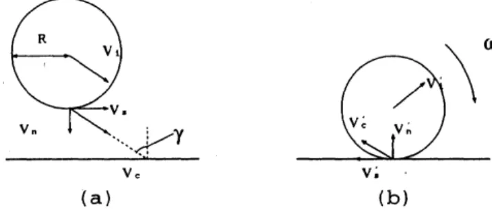
define the coefficient of restitution $\mathrm{e}$ and the coefficient of

tangentialrestitution $\beta$ in the 2-dimensional situation. Figure 1is the schematic figure that adisk

$\mathrm{v}_{\mathrm{c}}$

$\mathrm{t}$a I $\mathrm{t}\mathrm{b}$I

Figure 1: The schematic figure of acollision of sphere with awall.

is colliding with astationary wall with initialvelocity ofitscenter of mass, Vi. The relative velocity

at the contact point after collision, thus, becomes

$\mathrm{v}_{\mathrm{c}}’=\mathrm{v}_{\mathrm{i}}-R\mathrm{n}\mathrm{x}$ $\omega’$, (3)

where $R$ is the radius of the disk, $\mathrm{n}$ is the unit vector in the normal direction to the wall, and

$\omega$

’is

the angular velocity. The prime denotes post-colliding quantities. The coefficient of normal

restitution $\mathrm{e}$ is defined as

$\mathrm{v}_{\acute{\mathrm{c}}}\cdot \mathrm{n}=-e\mathrm{v}_{\mathrm{c}}\cdot \mathrm{n}$. (4)

Conventionally, this parameter is assumed to be $0\leq \mathrm{e}\leq 1$.

The coefficient of tangential restitution $\beta$ is defined

as

$\mathrm{v}_{\acute{\mathrm{c}}}\cdot \mathrm{t}=-\beta \mathrm{v}_{\mathrm{c}}\cdot \mathrm{t}$, (5)

where $\mathrm{v}_{\acute{\mathrm{c}}}$ and $\mathrm{t}$

are

the post-collisional velocity at the contact point after collision and the unit

tangential vector, respectively. It is believed that $\beta$ is afunction of the angle of incidence

$\gamma$, with

possible values lying in the

range

between -1 and 1 $[13, 14]$. The incident angle $\gamma$ is

defined

as

$\gamma=\arctan(\mathrm{v}_{t}/\mathrm{v}_{n})$, where $\mathrm{v}_{n}$ and $\mathrm{v}_{t}$

are

$\mathrm{v}_{n}=\mathrm{v}_{\mathrm{c}}\cdot$ $\mathrm{n}$ and $\mathrm{v}_{t}=\mathrm{v}_{\mathrm{c}}\cdot$

$\mathrm{t}$, respectively.

For the oblique collision, the coefficient of tangential restitution $\beta$ is more important than $e$.

From the conservation laws of momentum and angular momentum and Coulomb’s friction on tlte

surfaces of two identical $\mathrm{r}$igid

$\mathrm{s}\mathrm{l}$)

$1\mathrm{l}\mathrm{e}\mathrm{l}\mathrm{e}\mathrm{s}$, Walton[13] derives

$\beta\simeq\{$

$-1- \mu(1+e)\cot\gamma(1+\frac{mR^{\underline{)}}}{I})$ $(\gamma\geq\gamma_{0})$

$\beta_{0}$ $(\gamma\leq\gamma_{0})$,

(6)

where $\gamma_{0}$ is the critical angle, and $m$, $R$, and I

are

mass, radius and moment of inertia of spheres

respectively. Labous, Rosato, and Dave performed the experiment of binary collision of nylon

spheres and showed the consistency of their results to the Walton’s relation[14]. Furthermore, it

has become clear that Many experimental results

are

consistent with the relation

so

that Walton’s

model is accepted

as

reasonable[15, 16, 17]. Meanwhile, Maw, Barber, and Fawcett extended the

Hertz theory of impact and established the theory of the oblique impact to be consistent with

their experimental results[18]. In contrast to Walton’s assumption, they demonstrated the need to

consider normal and tangential compliance

over

the contact

area.

3Our

Models

Here, let

us

introduce three lattice models. Each model consists of

an

elastic disk and

an

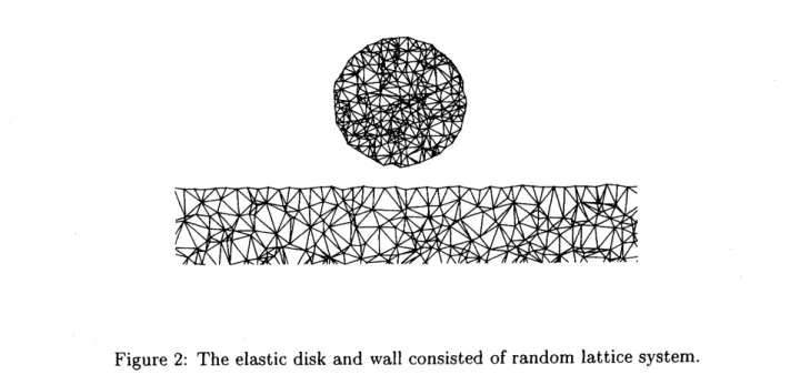
elastic

wall. The main results of this paper

are

those of random lattice model(Fig. 2). Both the disk and

Figure 2: The elastic disk and wall consisted ofrandom lattice system.

the wall

are

composed of randomly distributed 800

mass

points. All

mass

points

are

bound with

nonlinear springs using the Delaunay triangulation algorithm[19]. The spring interaction between

connected

mass

points is described

as

$V(x)= \frac{1}{2}k_{a}x^{2}+\frac{1}{4}k_{b}x^{4}$, (7)

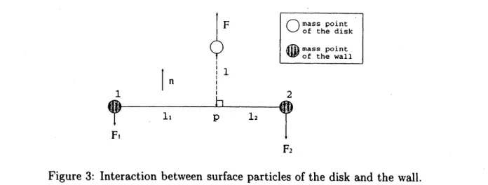
$\mathrm{F}_{-}$,

Figure

3:

Interaction between surface particles of the disk and the wall.

where $x$ is astretch from the natural length of spring, and $k_{a}$ and $k_{b}$

are

the spring constants. We

use

atypical ratio of $k_{b}$ to $k_{a}$

as

$k_{b}/k_{a}=10^{-3}$

.

The width of the wall is 4times

as

long

as

the

diameter ofthe disk. The height of the wall is

same

as

the diameter of the disk. Two sides of the

wall

are

fixed.

The interaction between the disk and the wallduring acollisionis introduced

as

follows. Figure

3isthe schematic figure of the interaction of surface

mass

points_{of the disk and the wall. When the}

distance $l$ between the edge of the disk and the surface ofthe wall is less than the cutoff

length(we

set it equal to the length of the linear spring), the surface particles of the disk feel the repulsive

force, $\mathrm{F}(l)=aV_{0}\exp(-al)\mathrm{n}$, where $a$ is $300/R$, $V_{0}$ is $amc^{2}R/2$, _$m$ is the

mass

of the particle, $R$

is the radius of the disk, $c=\sqrt{E}/\rho$, $E$ is Young’s modulus, and $\rho$ is the density, $\mathrm{n}$ is the normal

unit vector to the surface. The reaction forces applied to the two points of the surface of the

wall (point 1and 2)

are

decided by the balance of the torques

as

Fi$(/)=-F(l)\mathrm{n}/(1+/1//2)$ and

$\mathrm{F}_{2}(l)=-F(l)\mathrm{n}/(1+l_{2}/l_{1})$, where $l_{i}(i=1,2)$ is the distance between the point $p$ and the point $i$

(see Fig. 3).

In this model, roughness of the surfaces is important mechanism to make the disk rotate after

collision. How to make roughness is

as

follows. Atfirst,

we

generate normal random numbers whose

average

value is 0and then make the initial position of particles

on

surface of both the disk and

the wall deviate with them. We choose the value ofdispersion $\delta$

as

$\delta=3\cross 10^{-2}R$, where

$R$ is the

radius of the disk.

As for

random lattice model,

we

cannot

determine

Poisson’s ratio theoretically. When

we

determine Poisson’s

ratio of thismodel,

we

introduce the viscous damping term in (7). By stretching

the strip of random lattice and measuring its width and height,

we

can

obtain Poisson’s ratio.

Forcomparison,

we

make othertwo latticemodels: triangularlattice and square latticedisk(Fig.4).

The triangular lattice disk is made by replacing the internal structure of the random lattice disk

with the triangularlattice. The surface of the triangularlattice disk is

same as

that of the random

lattice disk. Poisson’s ratio ofthe triangular lattice

can

be calculated theoretically

as

1/3[20]. The

square lattice disk is made by replacing the internal structure of the random lattice disk with the

square lattice. We introduce two spring constants: $k_{a}=k_{1}$ for nearest neighbor interaction and

$k_{a}=k_{2}$ for next-nearest neighbor interaction. Poisson’s ratio of the

square

lattice is expressed

as

$\nu=\frac{k_{2}^{2}+(k_{1}^{2}-4k_{2}^{2})n_{x}^{2}n_{y}^{2}}{k_{2}(k_{1}+k_{2})+(k_{1}^{2}-4k_{2}^{2})n_{x}^{2}n_{y}^{2}}$

.

(8)

We scale the equation of motion for each particle using the radius of the

disk

$R$

as

the scale of

(a)

(b)

Figure 4: The schematic figures of (a) triangular lattice disk and (b) square lattice disk.

length and the velocity of elastic

wave

$c=\sqrt{E}/\rho$

as

the scaling unit ofvelocity.

As

the

numerical

scheme of the integration,

we use

the fourth order symplectic numerical method with the timestep

$\Delta t\simeq 10^{-3}R/c$.

4Results

and Discussions

In this section,

we

carry out the simulation ofthe oblique impact. The angle of incidence is ranged

from 5.7’ to80.5’ while the normal component ofvelocity is fixed

as

0.$1c$. Thedisk has

no

internal

vibration and rotation before collision. In order to eliminate the effect ofthe initial configuration

of

mass

points,

we

prepare

100

samples of disk

as

the initial condition by using

100

sets

of

random

numbers and average dataof all samples.

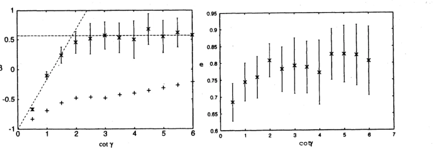
Figure 5: The relation between $\cot\gamma$ and $\beta$. Figure

6:

The relation between $\cot\gamma$ and $e$.

Figure 5shows the relation between the cotangent of the angle of incidence

7and

the coefficien$\mathrm{t}$

(9)

of tangential restitution $\beta$. In this figure,

cross

points

are

the result of the 1$\mathrm{a}\mathrm{n}\mathrm{d}\mathrm{o}\ln$ lattice disk

and $\backslash \backslash \prime \mathrm{a}11$, and broken lines

are

eq.(6), where

$e=0.8$, $\mu$ and $\beta_{0}$

are

fitting parameters. This result

shows that $\beta_{0}$ takes the value nearly 0.56 and $\mu_{0}$

takes

tlle value nearly0.18. From this estimation,

we can see that this model can reproduce the tendency _{of the experimental results of the oblique}

collision qualitatively$[14, 15]$. In contrast, plus points

are

the results ofthe triangular lattice disk.

In this lnodel, $\beta$ takes negative values in all range of the angle of incidence. This

means

that the

triangular lattice model is easy to slip on the surface.

Figure 6shows the relation between the cotangent of the angle of incidence and

COR

$e$.

Al-though it is expected that

COR

takes the constant value because the normal velocity ofthe disk is

set to the fixed value, 0.$1\mathrm{c}$,

COR

depends

on

the angle of incidence. In particular, in the region of

small value

of

$\cot\gamma$,

COR

decreases

as

$\cot\gamma$

decreases. At

present,

we

cannot explain this tendency

ofnormal

COR.

Here,

we

compare

our

result with the theory of Maw, et a1.[18]. According to their theory, all

the region of the angle of incidence

can

be divided into three regimes. For each regime, $\beta$

can

be

expressed

as

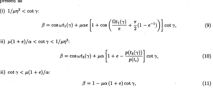
(i) $1/\mu\eta^{2}<\cot\gamma$:

$\beta=\cos\omega t_{1}(\gamma)+\mu\alpha e[1+\cos(\frac{\Omega t_{1}(\gamma)}{e}+\frac{\pi}{2}(1-e^{-1}))]\cot\gamma$,

(ii) $\mu(1+e)/\alpha<\cot\gamma<1/\mu\eta^{2}$:

$\beta=\cos\omega t_{3}(\gamma)+\mu\alpha[1+e-\frac{p(t_{3}(\gamma))}{p(t_{\mathrm{c}})}]\cot\gamma$, (10)

(iii) $\cot\gamma<\mu(1+e)/\alpha$:

$\beta=1-\mu\alpha(1+e)\cot\gamma$, (11)

where $\mu$ is the coefficient of friction, $\eta$ is the constant dependent

on

Poisson’s ratio, $\alpha=3.02$

which is aconstant dependent

on

the shape ofmaterial, $\Omega=\pi/2t_{c}$, $t_{/c}$ is aduration ofacollision,

$\omega$ $=(\pi/2\eta t_{c})\sqrt{\alpha}$, $t_{1}(\gamma)$ is thetransitiontime fromstickmotionto slip motion, $t_{3}(\gamma)$ is the transition

time from slip motion to stick motion, and $p(t)$ is impulse. This theory

was

confirmed to be

consistent with experimental data[15, 16, 17, 18].

We compare the result

of

simulation of theoblique impact using the random lattice model with

the theoretical curve(Fig. 7). Here

we

used $\eta=1.015$, which corresponds to Poisson’s ratio 0.058,

$e=0.8$

as

afixed value, and $\mu=0.3$

as

afitting parameter. It is found that the result of random

lattice model is consistent with the theory.

On the other hand,

as

for the result of figure 5,

we

focus

our

attention to the difference of

Poisson’s ratio between the random disk and the triangular disk. By changing the value of spring

constants of square lattice disk and controlling Poisson’s ratio,

we

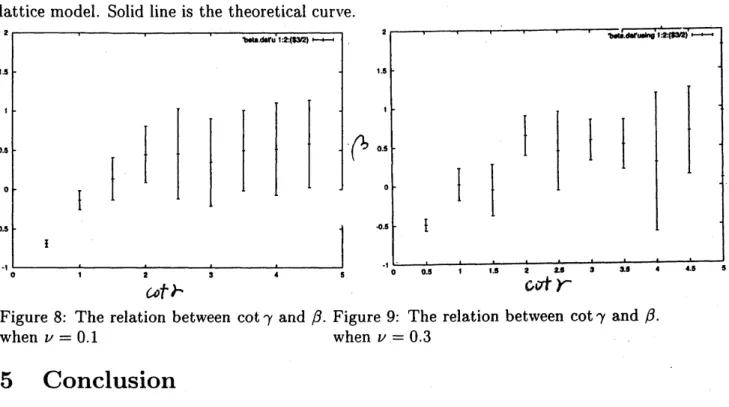
investigate the dependency of

$\beta_{0}$ on Poisson’s ratio. Figure 8is the result when $\nu=0.1$ while figure 9is the result when $\nu=0.3$.

We cannot

see

the difference of the values of$\beta_{0}$. From these results, Poisson’s ratio

seems

not to

affect the value of$\beta_{0}$

.

$\beta$

$\mathrm{c}\mathrm{o}q$

Figure 7: The relation between $\cot\gamma$ and $\beta$.

Cross

points

are

the numerical results of the random

lattice model. Solid line is the theoretical

curve.

A

Figure 8: The relation between $\cot\gamma$ and $\beta$. Figure 9: The relation between $\cot\gamma$ and $\beta$

.

when $\nu=0.1$ when $\nu=0.3$

5Conclusion

Inthis paper,

we

demonstrate the2-dimensional simulation of the oblique impactand obtain results

as

follows.

(i)

Our

random lattice model exhibits the

same

tendency

as

experimental data qualitatively. In

addition, the model is consistent with Maw’s theory of the oblique impact.

(ii) There

seems

to be

no

relation between Poisson’s ratio of material and the value of $\beta_{0}$.

References

[1] See, forexample, L. P. Kadanoff: Rev. Mod. Phys. 71 (1999) 435; P. G. de

Gennes:

Rev. Mod.

Phys. 71 (1999) S374 and references therein

[2] P. A. Cundall,

0.

D. L.

Strack:

Geotechnique 29 (1979) 47.

[3] I. Newton: Philoshophiae naturalis Principia mathematica (W. Dawason and Sons, London,

1962). The original

one

has been published in

1687.

[4] W. Goldsmith: Impa

ct:

The Theo

ry

and Physical Behavior

_of

Colliding

Solids

(Edward Arnold

Publ., London, 1960).

[5] K. L. Johnson: Contact Mechanics (Cambridge University Press, Cambridge, 1985).

[6] W. J. Stronge: Impact Mechanics (Cambridge Univ. Press, 2000)

[7] R. Sondergaard, K. Chaney, and

C.

E. Brennen: Transaction of theASME, Journal ofApplied

Mechanics

57

(1990)

694.

[8] F.

G.

Bridges,

A.

Hatzes, and

D.N.C.

Lin: Nature 309 (1984)

333.

[9] K. D. Supulver, F. G. Bridges, and D. N. C. Lin: ICARUS 113 (1995) 188

[10 G. Kuwabara and K. Kono: Jpn. J. Appl. Phys. 26 (1987) 1230.

[11 H. Hayakawa and H. Kuninaka: Chem. Eng.

Sci.

57 (2002)

239.

[12 M. Y. Louge and M. E. Adams: Phys. Rev. E65 (2002) 021303.

[13 O. R. Walton and R. L. Braun: J. Rheol. 30 (1986) 949.

[14 L. Labous, A. D. Rosato, and R. N. Dave: Phys. Rev. E56 (1997) 5717.

[15

S.

F. Foerster, M. Y. Louge, H. Chang, and K. Allia: Phys. Fluids 6(1994) 1108.

[16 A. Lorentz,

C.

Tuozzolo, and M. Y. Louge: Exp. Mech. 37 (1997) 292.

[17 D. A. Gorham, A. H. Kharaz: Powder Technology 112 (2000) 193.

[18 N. Maw, J. R. Barber, and J. N. Fawcett: Wear 38 (1976) 101.; N. Maw, J. R. Barber, and J.

N. Fawcett: ASME J. Lub. Tech 103 (1981) 74.

[19] K. Sugihara: Data Structure and Algorithms (Kyoritsu, Japan, 2001).

[20] W.

G.

Hoover: Computational Statistical Mechanics (Elsevier

Science

Publishers B. V.,

Ams-terdam, 1991