Coexistence states of a prey-predator model with population flux by attractive transition (Theory of Evolution Equation and Mathematical Analysis of Nonlinear Phenomena)
10
0
0
全文
(2) 163 term since Shigesada‐Kawasaki‐Teramoto [4] proposed a competition model with. cross‐diffusion terms to mathematically realize the segregation of two compet‐ ing species. For the prey‐predator relationship as (1.1), the cross‐diffusion term \alpha\triangle(uv) models an ecological situation that individuals of the prey diffuse from. the high density area to the low density area of the enemy (predator). Another is. the term \beta\nabla\cdot[u^{2}\nabla(v/u)] which is not widely known as the cross‐diffusion term in spite of the description parallel to the cross‐diffusion in the book by Okubo‐Levin. [3]. The nonlinear diffusion term \beta\nabla\cdot[u^{2}\nabla(v/u)] models an ecological situation. that individuals of the predator move towards the high density area of the feed. (prey). In the next section, following [3], we will explain reasons why such a couple. of nonlinear diffusion terms appear from the micro‐scopic modelling view‐point. Our interest is to derive the effect of nonlinear diffusion terms. onu. the set of. positive steady states. Then we will study the following stationary problem:. \{begin{ary}l d_{1}\triangleu+\alph triangle(uv)+ m_{1}-ucv)=0,x\inOmega, d_{2}\Deltav+\betanbl\cdot[u^{2}\nabl(\frac{v}u)]+v(m_{2}+bu-v)=0,x\in Omega, u=v0,x\inpartil\Omega, u\geq0,v\geq0,x\inOmega. \end{ary}. (1.2). On the linear diffusion system when \alpha=\beta=0 , there are a lot of papers (e.g., [5] and references therein) which study the set of positive solutions. The purpose of this article is to review some results obtained by the author’s joint researches ([1, 2]). The following four results about effects of nonlinear diffusion terms on positive solutions of (1.2) will be introduced. (i) A sufficient condition \mathcal{R}(\alpha, \beta) on the (m_{1}, m_{2}) plane for the existence of positive solutions.. (ii) The asymptotic behavior of \mathcal{R}(\alpha, \beta) as. \alphaarrow\infty.. (iii) The asymptotic behavior of \mathcal{R}(\alpha, \beta) as \betaarrow\infty.. (iv) In a special case when as. \alpha=0 ,. the asymptotic behavior of positive solutions. \betaarrow\infty.. The contents of this article is as follows: In Section 2, a mechanizm of nonlinear. diffusion terms of (1.1) will be explained from an ecological modelling viewpoint. In Section 3, we exhibits a sufficient region on the (m_{1}, m_{2}) plane for the existence of positive solutions (Fig. 2). In Section 4, the asymptotic behavior stated as above (ii)-(iv) will be introduced. Throughout this article, the usual norms of the spaces L^{p}(\Omega) for p\in[1, \infty ) and C(\overline{\Omega}) are defined by. \Vert u\Vert_{p}. :=( \int_{\Omega}|u(x)|^{p})^{1/p}. and. \Vert u\Vert_{\infty}. := \max_{x\in\overline{\Omega}}|u(x)|..
(3) 164. 2. Formulation of nonlinear diffusion in ecology. In this section, following the book by Okubo‐Levin [3], derivations of the cou‐ ple of nonlinear diffusion terms in (1.1) will be explained from the micro‐scopic modelling aspect. By the standard modelling procedure, we employ the ld‐spatio‐temporal dis‐ cretization such as. (x, t)=(n\triangle x,j\triangle t)\in \mathbb{R}\cross(0, \infty). ,. where n\in \mathbb{Z}, j\in \mathbb{N}\cup\{0\};\triangle x and \Delta t are tiny meshes for the space and time, respectively. In this setting, \{n\triangle x\}_{n\in Z} is assumed to be a one‐dimensional habitat of the prey and the predator, and each location n\triangle x is called n‐site. It is assumed that every individual of both species must to be positioned at some site n\Delta x and necessarily moves to either of neighbouring site (n-1)\triangle x or (n+1)\triangle x in a. unit time mesh \triangle t . Let u(x, t) (resp. v(x, t) ) be the number of individuals of the prey (resp. predator) at n‐site x=n\Delta x and time t=j\triangle t . Let T(m, n) be the transition probability of each individual from m\triangle x to. in time \triangle t , where. n\triangle x. |m-n|=1 (see Fig. 1). Under this setting, we estimate the difference of the. number of the prey at n‐site in time \triangle t by. u(x, t+\triangle t)-u(x, t)=T(n-1, n)u(x-\triangle x, t)+T(n+1, n)u(x+\triangle x, t) (2.1) -(T(n, n-1)+T(n, n+1))u(x, t) .. Figure 1: Transition rule. Here we derive the cross‐diffusion term (uv)_{xx} in the first equation of (1.1). For individuals of the prey, the low density location of the enemy (predator) is more favourable. So it is a natural situation that the transition probability T(m, n) of individuals of the prey depends on the number of the predator at departure site such as. Repulsive transition. T(m, n)= \frac{\triangle t}{(\triangle x)^{2} v(m\triangle x, t). (|m-n|=1) ,.
(4) 165 where \triangle t/(\triangle x)^{2} is related to the square root law for the Brownian motion. Sub‐. stituting this. T. into the recurrent formula (2.1), we obtain the differential quotient. \frac{u(x,t+\triangle t)-u(x,t)}{\triangle t}. = \frac{u(x+Ax,t)v(x+\triangle x,t)-2u(x,t)v(x,t)+u(x-\triangle x,t)v(x- \triangle x,t)}{(\Delta x)^{2} . By passing to the limit. \triangle tarrow 0. and \triangle xarrow 0 , we obtain the partial differential. equation. v_{t}=(uv)_{xx}. This is the one dimensional version of the cross‐diffusion part in (1.1).. Next we derive the nonlinear diffusion term (u^{2}(v/u)_{x})_{x} in the second equation. of (1.1). For individuals of the predator, the high density location of the feed (prey) is more favourable. Then it is reasonable to assume that the transition probability T(m, n) for individuals of t\dot{h}e predator depends on the number of the prey at arrival site such as Attractive transition. We substituting this. T. T(m, n)= \frac{\triangle t}{(\triangle x)^{2} u(n\triangle x,t). into (2.1) (with. u. (|m-n|=1) .. replaced by v) to obtain the differential. quotient. \frac{v(x,t+\triangle t)-v(x,t)}{\triangle t}=u(x, t)\frac{v(x+Ax,t)+v(x- \triangle x,t)-2v(x,t)}{(\triangle x)^{2} - \frac{u(x+Ax,t)+u(x-Ax,t)-2u(x,t)}{(\triangle x)^{2}}v(x, t) By the continuation procedure as \triangle tarrow 0 and \triangle xarrow 0 , we get the partial differential equation v_{t}=uv_{xx}-u_{xx}v , which is written by. v_{t}=(u^{2}( \frac{v}{u})_{x})_{x} This is the one dimensional version of the nonlinear diffusion part in the second. equation of (1.1).. In addition, we consider another model of T for the prey‐predator relation. It is also reasonable to assume that the transition probability T(m, n) of individuals. of the predator depends on the difference of feed (prey) between at arrival and at departure as follows: Transition by chemotaxis. T(m, n)= \frac{\triangle t}{2(\Delta x)^{2} (u(n\triangle x, t)-u(m\triangle x, t). ,.
(5) 166. Table 1. where |m-n|=1 . Substituting this. T. into (2.1) (with. u. replaced by v ), one can. see. \frac{v(x,t+\triangle t)-v(x,t)}{\triangle t}. =- \frac{u(x+\Delta x,t)+u(x-\triangle x,t)-2u(x,t)}{(\triangle x)^{2} \frac{v(x,t)+v(x-\triangle x,t)}{2} - \frac{u(x+\triangle x,t)-u(x,t)}{\triangle x}(\frac{v(x+\triangle x,t)-v(x,t) }{2\triangle x}+\frac{v(x,t)-v(x-\triangle x,t)}{2\triangle x}) By the continuation procedure, we get the partial differential equation -u_{xx}v-u_{x}v_{x} , which can be written as. .. v_{t}=. v_{t}=-(vu_{x})_{x}. This is an evolution equation driven by the so‐called chemotaxis term. These PDE modellings for typical three transitions of repulsive, attractive and difference types are generalized to the higher dimensional cases. We can summarize the correspondence table of transition type and nonlinear diffusion. and famous PDE models with such nonlinear diffusion terms (Table 1).. 3. Coexistence region. This section introduces a sufficient condition for the existence of positive solutions. of (1.2). In order to show a bifurcation aspect of the sufficient condition, we have to collect semitrivial solutions of (1.2). Here we call (u, v) a semitrivial solution of (1.2) if one of the components identically vanishes over \overline{\Omega} and the other is positive in \Omega . Ecologically, semitrivial solutions are corresponding to steady states such as one of the species becomes extinct and the other survives. If v vanishes over.
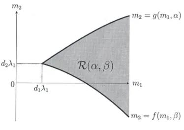
(6) 167 \overline{\Omega} , then. u. has to satisfy the following stationary logistic equation:. \{ begin{ar ay}{l} d_{1}\triangleu+u(m_{1}-u)=0 in\Omega, u=0 on\partial\Omega. \end{ar ay} It is well known that (3.1) admits a unique positive solution if and only if. (3.1) m_{1}>. -\triangle. d_{1}\lambda_{1} , where \lambda_{1} is the least eigenvalue of with homogeneous Dirichlet boundary condition on \partial\Omega . Then we denote the positive solution by \theta_{d_{1},m_{1} when ml > dı \lambda l.. Consequently, we see that (1.2) has a semitrivial solution (u, v)=(\theta_{d_{1},m1},0) if m_{1}>d_{1}\lambda_{1} . Similarly, one can verify that (1.2) has another semitrivial solution (u, v)=(0, \theta_{d_{2},m_{2}}) if m_{2}>d_{2}\lambda_{1}. A sufficient condition for the existence of positive solutions of (1.2) can be shown in the (mı, m_{2} ) plane as Fig. 2:. Theorem 3.1 ([1, 2]). If m_{1}\leq d_{1}\lambda_{1} , there is no positive solution of(1.2). In m_{1}>d_{1}\lambda_{1} , for any fixed. ca\mathcal{S}e. (d_{1}, d_{2}, b, c)\in \mathbb{R}_{+}^{4} , there exist two continuous functions. m_{2}=f(m_{1}, \beta) , m_{2}=g(m_{J}, \alpha) for. (m_{1}, \alpha, \beta)\in(d_{1}\lambda_{1}, \infty)\cros \overline{\mathbb{R} _ {+}^{2}. with. m \downar ow d_{1}\lambda_{1}\lim_{1}f(m_{1}, \beta)=\lim_{m_{1}\downar ow d_{1}\lambda_{1} g(m_{1}, \alpha)=d_{2}\lambda_{J} \lim_{m_{1arrow\infty} f(m_{1}, \beta)=-\infty and \lim_{m_{1arrow\infty} g(m_{1}, \alpha)=\infty ,. such that (1.2) admits at least one positive solution if. \min\{f(m_{1}, \beta), g(m_{1}, \alpha)\}<m_{2}<\max\{f(m_{1}, \beta), g(m_{1} , \alpha)\}. Let us explain the bifurcation aspect of Theorem 3.1. Regarding m_{2} as a real bifurcation parameter for any fixed m{\imath}>d_{1}\lambda_{1}, (u, v, m_{2})=(\theta_{d_{1},m_{1}},0, f(m], \beta)) and (u, v, m_{2})=(0, \theta_{d_{2},g(m_{1},\alpha)}, g(m_{1}, \alpha)) are bifurcation points from which positive solutions bifurcate. Furthermore, Theorem 3.1 ensures the existence of positive. solutions of (1.2) if (m_{1}, m_{2}) belongs to the surrounded region by two curves m_{2}=f(m_{1}, \beta) and m_{2}=g(m_{1}, \alpha) (see Fig. 2). It should be noted that f(m_{1}, \beta) (resp. g(m_{1}, \alpha) ) is independent of \alpha (resp. \beta ). Furthermore, in special cases when one of. \alpha. and \beta vanishes, the existence of a. bifurcation branch which connects these two semitrivial solutions was shown (see [1] for the case \beta=0;[21 for the other case \alpha=0 ). In this sense, the region. \mathcal{R}(\alpha, \beta):=\{(m_{1}, m_{2})\in(d_{1}\lambda_{1}, \infty)\cross \mathbb{R}| \min\{f(m_{1}, \beta), g(m_{1}, \alpha)\}<m_{2}<\max\{f(m_{1}, \beta), g(m_{1} , \alpha)\}\} exhibits a sufficient region for the existence of positive solutions..
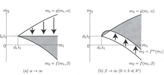
(7) 168 m_{2}. =g(m_{1}, \alpha). =f(m_{1}, \beta). Figure 2: A sufficient region for the existence of positive solutions of (1.2). 4. Asymptotic analysis as. \alphaarrow\infty. or \betaarrow\infty. In this section, we introduce the asymptotic behavior of \mathcal{R}(\alpha, \beta) as the nonlinear diffusion coefficient \alpha or \beta tends to infinity. In [1], the author and Yamada showed. the following dependence of \mathcal{R}(\alpha, \beta) on. \alpha>0. (see Fig. 3 (a) ).. Theorem 4.1 ([1]). For any fixed m_{1}>d_{1}\lambda_{1}, g(m_{1}, \alpha)\downarrow d_{2}\lambda_{1}a\mathcal{S}\alpha\uparrow\infty . In other words, it hold_{\mathcal{S}} that. \lim_{\alphaarrow\infty}\mathcal{R}(\alpha, \beta)=\{(m_{1}, m_{2})\in(d_{1} \lambda_{1}, \infty)\cross \mathbb{R}| \min\{f(m_{1}, \beta), d_{2}\lambda_{1} \} <m_{2}<\max\{f(m_{1}, \beta), d_{2} \lambda_{1} \} \}. In [2], Oeda and the author obtained the following asymptotic behavior of \mathcal{R}(\alpha, \beta) as \betaarrow\infty (see Fig. 3 (b)). Theorem 4.2 ([2]). It holds true that. \lim_{\beta r ow\infty}\mathcal{R}(\alpha, \beta). :=\{(m_{1}, m_{2})\in ( d_{1}\lambda_{1} , oo) \cross \mathbb{R}|. \min\{f^{\infty} (m_{1} ), g(m_{1}, \alpha)\}<m_{2}<\max\{f^{\infty}(m_{1} ), g(m_{1}, \alpha)\}\}, where. f^{\infty}(m_{1}):= \lim_{\alpha r ow\infty}f(m_{i}, \alpha)=\frac{d_{2} {d_{ \imath} m_{1}-(\frac{d_{2} {d_{1} +b)\frac{|\theta_{d_{1},m_{1} |_{2} ^{2} {|\theta_{d_{1},m_{1} |_{1} ..
(8) 169 \alpha). \alpha). f^{\infty}(m_{1}) \beta). \beta). (a). ( b ) \betaarrow\infty(0<b\ll b^{*}). \alphaarrow\infty. Figure 3: Asymptotic behaviors of \mathcal{R}(\alpha, \beta) stated in Theorems 4.1 and 4.2. We note the following asymptotic profile of f^{\infty}(m_{1}) as m_{1}\downarrow d_{1}\lambda_{1} and. m_{1}arrow\infty. obtained in [2]:. \lim_{m_{1}\downar ow d_{1}\lambda_{1} f^{\infty}(m_{1})=d_{2}\lambda_{1},. \frac{d}{dm_{1} f^{\infty}(d_{J}\lambda_{1}):=\lim_{m_{1}\downar ow d_{1} \lambda_{1} \frac{d}{dım} f^{\infty}(m_{1})= \frac{d_{2} {d_{1} -(\frac{d_{2} {d_{1} +b)\frac{1} {\Vert\Phi\Vert_{1}\Vert\Phi\Vert_{3}^{3} ,. (4.1). \lim_{m_{1arrow\infty} f^{\infty}(m_{1})=-\infty,. where. \Phi. is the positive function satisfying -\triangle\Phi=\lambda_{1}\Phi. in. \Omega,. \Phi=0 on. \partial\Omega,. \Vert\Phi\Vert_{2}=1.. Since it is verified that \Vert\Phi\Vert_{1}\Vert\Phi\Vert_{3}^{3}>1 by the Schwarz inequality, then (4.1) gives. \frac{d}{dm_{1}f^{\infty}(d_{1}\lambda_{1})\{ begin{ar ay}{l} >0 if0<b ^{*}:=\frac{d_{2}{d_{1}(\Vert\Phi\Vert_{1}\Vert\Phi\Vert_{3}^{3}- 1), <0 ifb> ^{*} \end{ar ay} Therefore, when 0<b<b^{*} , the curve m_{2}=f^{\infty}(m_{1}) is monotone increasing if m_{1}-d_{1}\lambda_{1}>0 is sufficiently small whereas it is monotone decreasing if m_{1}>0 is sufficiently large. In the special case when \alpha=0 , we get the following limiting characterization of positive solutions as \betaarrow\infty . The following result gives the asymptotic behavior. of positive solutions of (1.2) as. \alphaarrow\infty..
(9) 170 Theorem 4.3 ([2]). Suppose that. \alpha=0. and (m_{1}, m_{2}, d_{1}, d_{2}, b, c) satisfies. m_{1}>d_{1}\lambda_{1},. m_{2}\neq f^{\infty}(m_{1}). ,. m_{2} \neq\frac{d_{2} {d_{1} m_{1}-(\frac{d_{2} {d_{1} -\frac{1}{c}) \frac{|\theta_{d_{1},m_{1} |_{2}^{2} {|\theta_{d_{1},m_{1} |_{1} (=:h(m_{1}) ) m_{2}\neq g(m_{1},0). ,. .. Let \{(u_{n}, v_{n})\} be any sequence of positive solutions to (1.2) with. \alpha=0. \beta_{n}arrow\infty . Then the following alternative holds true.. and \beta=. (i) If \{\beta_{n}\Vert u_{n}\Vert_{\infty}\} is unbounded, then f^{\infty}(m_{1})<m_{2}<h(m_{1}) . In this case, for s\in(0,1) defined by m_{2}=(1-s)f^{\infty}(m_{1})+sh(m_{1}). ,. there exists a subsequence of \{(u_{n}, v_{n})\} (which is denoted by \{(u_{n}, v_{n})\} again) \mathcal{S}uch that. \lim_{nar ow\infty}(u_{n}, v_{n})=(1-s, \frac{s}{c})\theta_{d_{1},m_{1}. in. C^{1}(\overline{\Omega})\cros C^{1}(\overline{\Omega}). .. (ii) If \{\beta_{n}\Vert u_{n}\Vert_{\infty}\} is bounded, there exists (w, v)\in C^{2}(\overline{\Omega})\cross C^{2}(\overline{\Omega}) such that. \lim_{narrow\infty}(\beta_{n}u_{n}, v_{n})=(w, v). in. C^{1}(\overline{\Omega})\cros C{\imath} (\overline{\Omega}). ,. passing to a subsequence, and moreover, (u), v ) is a positive solution to. \{begin{ar y}{l d_{1}\trianglew+ (m_{1}-cv)=0, x\inOmega, d_{2}\trianglev+\nabl\cdot[w^{2}\nabl(\frac{v}w)]+v(m_{2}-v)=0, x\inOmega, w=v0, x\inpartil\Omega. \end{ar y} In the first situation (i) of Theorem 4.3, the set. \{(u, v, m_{2})=( 1-s, \frac{\mathcal{S} {c})\theta_{d_{1)}m_{1} , (1-s) f^{\infty}(m_{1})+sh(m_{1}) 0<\mathcal{S}<1\} of limit functions forms aline connects. (\theta_{d_{1},m_{1}},0, f^{\infty}(m_{1})) with (0, \theta_{d_{1},m_{1}}/c, h(m_{1})) . We should note that any (u, v) on this line satisfies the following limiting system of.
(10) 171 171. (1.2) as \beta_{n}arrow\infty which consists of the equal diffusive Lotka‐Volterra competition equations and an integral equation:. \{begin{ary}l d_{1}\triangleu+(m_{1}-ucv)=0,x\inOmega, d_{1}\trianglev+(m_{1}-ucv)=0,x\inOmega, u=v0,x\inpartl\Omega, \frc{d_2} {1\int_{Omega}v(m{\iath}-ucv)=\int_{Omega}v(m_{2}+bu- v). \end{ary}. (4.2). By Theorem 4.3, one can expect that almost all positive solution of (1.2) with large \beta can be characterized by either of type (i) or (ii). In view of the first type (i), the coexistence steady state (u, v) of prey and predator can be approximated by a coexistence steady state of the equal diffusive competition model (4.2) with an integral constraint. On the other hand, in the second type (ii), the component of prey shrinks with order O(1/\beta) when \beta is sufficiently large.. References [1] K. Kuto, Y. Yamada, Positive solutions for Lotka‐Volterra competition sys‐ tems with large cross‐diffusion, Appl. Anal., 89 (2010), 1037‐1066.. [2] K. Oeda, K. Kuto, Positive steady states for a prey‐predator model with pop‐ ulation flux by attractive transition, submitted.. [3] A. Okubo, L. A. Levin, Diffusion and Ecological Problems: Modern Perspec‐ tive, Second edition. Interdisciplinary Applied Mathematics, 14, Springer‐ Verlag, New York, 2001.. [4] N. Shigesada, K. Kawasaki, E. Teramoto, Spatial segregation of interacting species, J. Theor. Biol., 79 (1979), 83‐99.. [5] Y. Yamada, Stability of steady states for prey‐predator diffusion equations with homogeneous Dirichlet conditions, SIAM J. Math. Anal., 21 (1990), 327‐ 345.. Graduate School of Informatics and Engineering The University of Electro‐Communications 1‐5‐1 Chofugaoka, ChofU‐shi, Tokyo 182‐8585, JAPAN E‐mail address: k‐[email protected].
(11)
図
関連したドキュメント
The system evolves from its initial state without being further affected by diffusion until the next pulse appears; Δx i x i nτ − x i nτ, and x i nτ represents the density
Complex formation is used as a unified approach to derive represen- tations and approximations of the functional response in predator prey relations, mating, and sexual
It is suggested by our method that most of the quadratic algebras for all St¨ ackel equivalence classes of 3D second order quantum superintegrable systems on conformally flat
In particular, we consider a reverse Lee decomposition for the deformation gra- dient and we choose an appropriate state space in which one of the variables, characterizing the
Pioneering works on the existence of traveling wave solutions connecting two steady states (point-to-point orbit) for diffusive predators-prey systems (1.2) are found in Dunbar [6,
From the second, third and fourth rows, we assert that predator–prey systems with harvesting rate on the prey species have similar dynamical behav- iors around its positive
This paper presents an investigation into the mechanics of this specific problem and develops an analytical approach that accounts for the effects of geometrical and material data on
We study the classical invariant theory of the B´ ezoutiant R(A, B) of a pair of binary forms A, B.. We also describe a ‘generic reduc- tion formula’ which recovers B from R(A, B)
