FROM CONVEX POLYTOPES TO MULTI-POLYTOPES (Algebraic Combinatorics on Convex Polytopes)

(1)

FROM CONVEX POLYTOPES TO MULTI-POLYTOPES

Osaka

City University Mikiya Masuda (枡田幹也)

1. INTRODUCTION

We introduce the notion of multi-polytopes generalizing that of

convex

polytopes, and

report that Ehrhart polynomials and Khovanskii-Pukhlikov

on

lattice

convex

polytopes

(i.e.,

convex

polytopes with vertices in the lattice) can be extended to lattice

multi-polytopes. This is ajoint work with A. Hattori and the detailed argument and

a

connec-tion with geometry

can

be found in [7].

Let

us

briefly explain the idea ofmulti-polytopes. It

comes

from geometry. According

to the theory of toric varieties,

a

lattice

convex

polytope $P$ corresponds to

an

ample line

bundle $L$ over a compact non-singular toric variety $M$. In fact, $P$ is the image of $M$ by

the moment map associated with $L$. This suggests

us

to view the

convex

polytope $P$

as

being formed from two combinatorial data corresponding to $M$ and $L$. We shall explain

them for

a convex

polygon (i.e., two-dimensional

convex

polytope) $P$ shown in Figure

1(1). We take an (outward) normal vector to each side and form four two-dimensional

cones, each of which isspanned by two normal vectors whose corresponding sides intersect

at a vertex of $P$. Then we obtain a complete fan shown in Figure 1(2). This complete

fan is the combinatorial datum corresponding to the base space $M$ in the theory oftoric

varieties. The other datum is

an

arrangement oflines obtained by extending the sides of

$P$,

see

Figure 1(3). This arrangement is the information brought by the line bundle $L$.

Note that the arrangement is related to the fan. Namely the lines in the arrangement

are

perpendicular to the edge vectors in the fan.

$(|)$

’ _{$(s_{b})$}

$\mathrm{E}^{1}\mathrm{I}\mathrm{G}\mathrm{U}\mathrm{R}\mathrm{E}1$

The observation above

can

be applied to $n$-dimensional

convex

polytopes. In thiscase,

the associated fan is

an

$n$

-dimensional

completefan andthearrangement consists ofaffine

hyperplanes in an $n$-dimensional vector space which

are

perpendicular to edge vectors in

the fan.

Now, let

us

take the followingstar shaped figure $Q$ and make the

same

observation

as

(2)

FIGURE 2

Then

we

obtain five two-dimensional cones, each of which is spanned by two normal

vectors whose corresponding sides intersect at

a

vertex. A notable fact is that the

cones

have overlap and the degree of overlap is uniformly two. This is

an

example of almost

what

we

call

a

complete multi-fan. The multi-polytope associated with $Q$ is

a

pair of the

complete multi-fan and the arrangement oflines obtained by extending the five sides of

$Q$. In general,

a

multi-polytope is defined to be

a

pair of

a

complete multi-fan and

an

arrangement ofaffine hyperplanes perpendicular to edge vectors in the multi-fan.

This article is organized

as

follows. In section 2

we

give

a

precise definitionof multi-fan

and multi-polytope. We also define the notion of completeness, simpliciality and

non-singularity of

a

multi-fan. The definition of simpliciality and non-singularity is

straight-forward but the definition ofcompleteness is somewhat complicated and essential in

our

argument. In section 3

we

associate with

a

simple multi-polytope

an

interger valued

lo-cally constant function (called the Dusitermaat-Heckman function) on the complenent of

the hyperplane arrangement. When the multi-polytope arises from

a

convex

polytope $P$,

the function takes 1

on

the interior of$P$ and $0$ on the otherregions divided by the

hyper-plane arrangement. The generalization of Ehrhartpolynomials andKhovanskii-Pukhlikov

formula is discussed in sections 4 and 5 respectively.

2. MULTI-FANS AND MULTI-POLYTOPES

In this section,

we

define

a

multi-fan which is

a

complete generalization of

a

fan

and introduce the notion ofmulti-polytopes. We also define the completeness and

non-singularity of

a

multi-fan generalizing the corresponding notion of

a

fan. We shall begin

with reviewing the definition of

a

fan.

Let $N$ be

a

lattice of rank $n$, which is isomorphic to $\mathbb{Z}^{n}$. We denote the real vector space $N\otimes \mathbb{R}$ by $N_{\mathbb{R}}$. A subset $\sigma$ of$N_{\mathbb{R}}$ is called

a

strongly

convex

rational polyhedral

cone

(with apex at the origin) if there exits

a

finite number of vectors $v_{1},$_$\ldots,$$v_{m}$ in $N$ such

that

$\sigma=$

{

$r_{1}v_{1}+\cdots+r_{m}v_{m}|r_{i}\in \mathbb{R}$and $r_{i}\geq 0$ for all $i$

}

and $\sigma\cap(-\sigma)=\{0\}$. Here “rational”

means

that it is generated by vectors in the lattice

$N$, and “strong” convexity that it contains

no

line through the origin. We will often call

a

strongly

convex

rational polyhedral

cone

in $N_{\mathbb{R}}$ simply

a cone

in $N$. The dimension

$\dim\sigma$ of

a

cone

a is the dimension of the linear space spanned by vectors in

$\sigma$. A subset $\tau$ of a is called

a

face

of $\sigma$ if there is

a

linear function $\ell:N_{\mathbb{R}}arrow \mathbb{R}$ such that $p$ takes

(3)

nonnegative values

on

a and $\tau--\ell^{-1}(0)\cap\sigma$. A

cone

is regarded

as a

face of itself, while

others

are

calledproper faces. Definition. A fan $\triangle$ in $N$ is a set

of

a

finite number of strongly

convex

rational

polyhe-dral

cones

in $N_{\mathbb{R}}$ such that

(1) Each face of

a

cone

in $\triangle$ is also

a

cone

in $\triangle$;

(2) The intersection oftwo

cones

in $\Delta$ is

a

face ofeach, (so

that different

cones

do not

overlap).

Definition. A fan $\triangle$

is said to be complete if the union of

cones

in $\triangle \mathrm{c}\mathrm{o}$

,

vers

$\mathrm{t}\mathrm{h}\mathrm{e}arrow$ entire

space $N_{\mathbb{R}}$.

A

cone

is called simplicial,

or a

simplex, if it is generated by linearly independent

vectors. Ifthe generating vectors

can

be taken

as a

$.\mathrm{p}$art of

a

$\mathrm{b}.$

asi.s

o..f

$N,$

th.en

the

con..e

is called non-singular.

Definition. A fan $\triangle$ is said to be simplicial

(resp. non-singular) ifevery

cone

in $\Delta$ is

simplicial (resp. non-singular).

The

fundamental

fact in the theory of toric varieties says that there is

a

$\mathrm{o}\mathrm{n}\mathrm{e}- \mathrm{t}_{0}$

-one

correspondence between $n$-dimensional toric varieties and $n$-dimensional fans, and

a

fan

is complete (resp. simplicial

or

non-singular) if and only if the corresponding

_toric.

variety

is compact (resp.

an

orbifold

or

non-singular).

Foreach$\tau\in\triangle$,

we

define $N^{\tau}$ to be the quotientlattice of_$N$ by

the sublattice generated

(as

a

group) by$\tau\cap N$;

so

the rankof$N^{\tau}$ is$n-\dim\tau$. Weconsider

cones

in $\triangle$ that

contain

$\tau$

as a

face, and project them

on

$(N^{\mathcal{T}})_{\mathbb{R}}$. These projected

cones

form

a

fan in $N^{\tau}$, which

we

denote by $\triangle_{\tau}$ and call the projected

fan

with respect to $\tau$. The dimensions of the

projected

cones

decrease by $\dim\tau$. The completeness, $\mathrm{s}\mathrm{i}\mathrm{m}_{\mathrm{P}^{1}}\mathrm{i}\mathrm{c}\mathrm{i}\mathrm{a}\mathrm{l}\mathrm{i}\mathrm{t}\mathrm{y}$

. $\mathrm{a}.\mathrm{n}$ . $\mathrm{d}.\mathrm{n}$on-sing $\mathrm{t}$

ular..ity

of$\triangle$ will

be inherited to $\triangle_{\tau}$ for any

$\tau$.

We

now

generalize these notions of

a

fan. Let $N$ be

as

before. Denote by _$C(N)$ the

set of all

cones

in $N$. An ordinary fan is

a

subset of _$C(N)$. The set _$C(N)$ has

a

(strict)

partial $\mathrm{o}\mathrm{r}\mathrm{d}\mathrm{e}\mathrm{r}\mathrm{i}\mathrm{n}\mathrm{g}\prec \mathrm{d}\mathrm{e}\mathrm{f}\mathrm{i}\mathrm{n}\mathrm{e}\mathrm{d}$ by: $\tau\prec\sigma$ if and only if$\tau$ is

a

proper face of$\sigma$. The

cone

$\{0\}$

consisting of the origin is the unique minimum element in $C(N)$. On the other hand, let

$\Sigma$ be

a

partially ordered finite set with

a

unique minimum element. We denote by the

(strict) partial ordering by $<$ and the minimum element by $*$. An example of $\Sigma$ used

later is

an

abstract simplicial set with

an

empty set added

as a

member, which

we

call

an

augmented simplicial set. In this

case

the partial ordering is defined by the inclusion

relation and the empty set is the unique minimum element which may be considered

as

a

$(-1)$-simplex. Suppose that there is a _map

$\Lambda:\Sigmaarrow C(N)$ such that

(1) $\Lambda(*)=\{0\}$;

(2) If $I<J$ for $I,$ $J\in\Sigma$, then $\Lambda(I)\prec\Lambda(J)$;

(3) For any $I,$ $J\in\Sigma$ and $\kappa\in C(N)$ such that $I<J$ and $\Lambda(I)\prec\kappa\prec\Lambda(J)$, there is

a

unique element $K\in\Sigma$ such that

$I<K<J$

and _{$\Lambda(K)=\kappa$}.

For

an

integer $m$ such that $0\leq m\leq n$,

we

set

(4)

One

can

easilycheck that $\Sigma^{(m)}$ does not depend

on

A. When $\Sigma$ is

an

augmented simplicial

set, $I\in\Sigma$ belongs to $\Sigma^{(m)}$ if and only if the cardinality $|I|$ of $I$ is $m$, namely $I$ is

an

$(m-1)$-simplex. Therefore,

even

if $\Sigma$ is not

an

augmented simplicial set,

we

use

the

notation $|I|$ for $m$ when $I\in\Sigma^{(m)}$.

The image $\Lambda(\Sigma)$ is

a

finite set of

cones

in $N$. We may think of

a

pair $(\Sigma, \Lambda)$

as a

set of

cones

in $N$ labeled by the ordered set $\Sigma$. Cones in

an

ordinary fan intersect only at their

faces, but

cones

in $\Lambda(\Sigma)$ may overlap,

even

the

same cone

may appear repeatedly with

different labels. The pair $(\Sigma, \Lambda)$ is almost what

we

call

a

multi-fan, but

we

incorporate

a pair of weight functions on

cones

in $\Lambda(\Sigma)$ of the highest dimension $n=\mathrm{r}\mathrm{a}\mathrm{n}\mathrm{k}N$. More

precisely, we consider two functions

$w^{\pm}:$ $\Sigma^{(n)}arrow \mathbb{Z}_{\geq 0}$.

These two functions naturallyarise from geometry, and their

sum

corresponds to $\mathrm{E}\mathrm{u}\mathrm{l}\mathrm{e}\mathrm{r}\backslash$

number while their difference is related to Todd genus (see [10]).

Definition. We call a triple $\triangle:=(\Sigma, \Lambda, w^{\pm})$

a

multi-fan

in $N$. We define the dimension

of$\triangle$ to be the rank of $N$ (or the dimension of$N_{\mathbb{R}}$).

Since

an

ordinary fan $\triangle$ in $N$ is

a

subset of $C(N)$,

one

can view it

as

a multi-fan by

taking $\Sigma=\triangle,$ $\Lambda=\mathrm{t}\mathrm{h}\mathrm{e}$ inclusion map, $w^{+}=1$, and $w^{-}=0$. In

a

similar way

as

in the

case

of ordinary fans,

we

say that

a

multi-fan $\triangle=(\Sigma, \Lambda, w^{\pm})$ is simplicial (resp.

non-singular) ifevery

cone

in $\Lambda(\Sigma)$ is simplicial (resp. non-singular). The following lemma is

easy.

Lemma 2.1. A

_multi-fan

$\triangle=(\Sigma, \Lambda, w^{\pm})$ is simplicial

if

and only

if

$\Sigma$ is isomorphic to

an $au.,gm_{\mathrm{I}}e$nted

si.m

p..l.ic.

$ial$

: set as

$p.artia\iota l\backslash \backslash \cdot y$

o.rdered

sets.

$\mathrm{r}$ Thedefinition ofcompletenessof

a

multi-fan

$\triangle$israther complicated. Anaivedefinition

of the completeness would be that the union of

cones

in $\Lambda(\Sigma)$

covers

the entire space

$N_{\mathbb{R}}$. But this is not

a

right definition. Although the two weighted functions

$w^{\pm}$ are

incorporated in the definition of

a

multi-fan, only the difference

$w:=w^{+}-w^{-}$

matters in this article. We shall introduce the following intermediate notion of

pre-completeness at first.

Definition. We call a multi-fan $\triangle=(\Sigma, \Lambda, w^{\pm})$ pre-complete if the integer

$v \in\Lambda\sum_{(I)}w\{I)$

is independent ofthe coice of

a

generic element$v$ in $N$. Here the sum above is understood

to be

zero

if there is

no

such$I$, and “generic”

means

that$v$doesnot lie

on

alinear subspace

spanned by

a cone

in $\Lambda(\Sigma)$ ofdimension less than $n$. We callthe integer above the degree

of$\triangle$ and denote it by _{$\deg(\triangle)$}.

Remark. For

an

ordinary fan, pre-completeness is

same as

completeness.

To define the completeness for a multi-fan $\triangle$,

we

need to define

a

projected multi-fan

with respect to

an

element in $\Sigma$. We do it

as

follows. For each $K\in\Sigma$, we set

(5)

It inherits the partial ordering from $\Sigma$, and $K$ is the unique minimum element in $\Sigma_{K}$. A

map

$\Lambda_{K}$: $\Sigma_{K}arrow C(N^{\Lambda(K)})$

sending $J\in\Sigma_{K}$ to the

cone

$\Lambda(J)$ projected

on

$(N^{\Lambda(K)})_{\mathbb{R}}$ satisfies the three properties

above required for A. We define two functions

$w_{K^{\pm}}:$ $\Sigma_{K^{-|K|)}}^{(n}\subset\Sigma^{(n)}arrow \mathbb{Z}_{\geq 0}$

to be the restrictions of $w^{\pm}$ to $\Sigma^{(n}K-|K|$). A triple $\triangle_{K}:=(\Sigma_{K}, \Lambda_{K}, W_{K^{\pm}})$ is

a

multi-fan in

$N^{\Lambda(K)}$, and this is the desired projected

multi-fan

with respect to _$K\in\Sigma$. When $\triangle$ is

an

ordinary fan, this definition agrees with the previous

one.

Definition. A pre-complete multi-fan $\triangle=(\Sigma, \Lambda, w^{\pm})$ is said to be complete if the

pro-jected multi-fan $\triangle_{K}$ is pre-complete for any $K\in\Sigma$.

Example 2.2. Here is an example of

a

complete non-singular multi-fan of degree two.

Let $v_{1},$_$\ldots,$$v_{5}$ be integral vectors shown in the following figure, where the dots denote

la..ttice

points.

$q\}_{\Omega}$ $?)_{A}$

$\mathrm{u}_{5}$ $\mathrm{u}_{\mathrm{d}}$

FIGURE 3

The vectors

are

rotating around the origin twice in counterclockwise. We take

$\Sigma=\{\phi, \{1\}, \ldots, \{5\}, \{1,2\}, \{2,3\}, \{3,4\}, \{4,5\}, \{5,1\}\}$, define $\Lambda:\Sigmaarrow C(N)$ by

$\Lambda(\{i\})=$ the

cone

spanned by $v_{i}$,

$\Lambda(\{i, i+1\})=$ the

cone

spanned by $v_{i}$ and $v_{i+1}$,

where $i=1,$$\ldots$ ,5 and 6 is understood to be 1, and take

$w^{\pm}$ such that $w=1$ on every

two dimensional

cone.

$\mathrm{T}\mathrm{h}\mathrm{e}\mathrm{n}_{1},\triangle=(\Sigma, \Lambda, w^{\pm})$ is

a

comp.l.ete

non-singul.ar

two-dimensional

multi-fan with $\deg(\triangle)=2$.

Examp.le

2.3. Here is an example of a complete multi-fan “with folds”. Let $v_{1},$ _$\ldots,$$v_{5}$

be vectors shown in $\mathrm{t}\dot{\mathrm{h}}\mathrm{e}\mathrm{f}\mathrm{o}\mathrm{l}\dot{\mathrm{l}}\mathrm{o}\mathrm{W}\mathrm{i}\mathrm{n}\mathrm{g}$ figure.

We define $\Sigma$ and A

as

in Example 2.2 and take $w^{\pm}$ such that

$w(\{3,4\})=-1$ and $w(\{i, i+1\})=1$ for $i\neq 3$.

(6)

$\nwarrow \mathrm{r}$

.

$\bigvee_{3}$

FIGURE 4

A similar example

can

be constructed for

a

number of vectors $v_{1},$ _$\ldots,$$v_{d}(d\geq 2)$ by

defining

$w(\{i, i+1\})=1$ if$v_{i}$ and $v_{i+1}$

are

rotating in counterclockwise,

$w(\{i, i+1\})=-1$ _if$v_{i}$ and $v_{i+1}$

are

rotating in clockwise,

where $d+1$ is understood to be 1. The degree $\deg(\triangle)$ is the rotation number of the

vectors $v_{1},$$\ldots$ ,$v_{d}$ around the origin in counterclockwise and may not be

one.

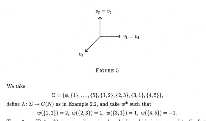
Example 2.4. Here is

an

exampleof

a

multi-fanwhich is pre-complete but not complete.

Let $v_{1},$

$\ldots,$$v_{5}$ be vectors shown in the followingfigure.

$v_{2}=v_{5}$

FIGURE 5

We take

$\Sigma=\{\phi, \{1\}, \ldots, \{5\}, \{1,2\}, \{2,3\}, \{3,1\}, \{4,5\}\}$, define $\Lambda:\Sigmaarrow C(N)$

as

in Example 2.2, and take $w^{\pm}$ such that

$w(\{1,2\})=2,$ $w(\{2,3\})=1,$ $w(\{3,1\})=1,$ $w(\{4,5\})=-1$.

Then $\triangle=(\Sigma, \Lambda, w^{\pm})$ is a two-dimensional multi-fan which is pre-complete (in fact,

$\deg(\triangle)=1)$ but not complete because the projected multi-fan $\triangle\{i\}$ for $i\neq 3$ is not

pre-complete.

So far,

we

treated rational

cones

that

are

generated by $\backslash ’\cdot \mathrm{e}\mathrm{c}\mathrm{t}\mathrm{o}\mathrm{r}\mathrm{S}$ in the lattice $N$. But,

most of the notions introduced above make

sense even

if

we

allow

cones

generated by

(7)

lattice $N$, but others do not. Therefore,

one can

define

a

multi-fan and its completeness

and simpliciality in this extended category

as

well. In

_t.he

following

we

will denote $N_{\mathbb{R}}$

by $V$.

As explained in the introduction,

a convex

polytope

or

the star shaped figure produces

a

complete multi-fan and

an

arrangement of hyperplanes perpendicular to edge vectors

in the multi-fan. Taking this observation into account,

we reverse a

gear. We start with

a

complete multi-fan $\triangle=(\Sigma, \Lambda, w^{\pm})$. It is convenient to think of the hyperplanes

as

sitting in the dual space $V^{*}$ of$V$. Let HP$(V^{*})$ be the set of all affine hyperplanes in $V^{*}$.

Definition. Let $\triangle=(\Sigma, \Lambda, w^{\pm})$ be

a

complete multi-fan and let $F:\Sigma^{(1)}arrow \mathrm{H}\mathrm{P}(V^{*})$ be

a

map such that the affine hyperplane $F(J)$ is ‘perpendicular’ to the half line $\Lambda(J)$ for

each $J\in\Sigma^{(1)}$, i.e.,

an

element in _$\Lambda(J)$ takes

a

constant

on

_$F(J)$. We call

a

pair $(\triangle, \mathcal{F})$

a

multi-polytope and denote it by $P$. The dimension of

a

multi-polytope $P$ is defined to

be the dimension of the multi-fan $\triangle$. We say that

a

multi-polytope

$P$ is simple if $\triangle$ is

simplicial. When $P$ is simple, $\bigcap_{i\in I}\mathcal{F}(\{i\})$ for $I\in\Sigma^{(n)}$ is called

a

vertex of$P$, and if all

vertices of$P$

are

lattice points, then

we

say that $P$ is

a

simple lattice multi-polytope.

Remark. There are two notions similar to that of multi-polytopes, which

were

introduced

byKarshon-Tolman [8] andKhovanskii-Pukhlikov [9] when $\triangle$ is

an

ordinaryfan. They

use

the terminology twisted polytope and virtual polytope respectively. The notion of

multi-polytopes is

a

direct generalization of that oftwisted polytopes, and also generalizesthat

of virtual polytopes,

see

[11].

3.

$\mathrm{D}\mathrm{u}\mathrm{I}\mathrm{s}\mathrm{T}\mathrm{E}\mathrm{R}\mathrm{M}\mathrm{A}\mathrm{A}\mathrm{T}$-HECKMAN

FUNCTIONS

A multi-polytope $P=(\triangle, F)$ defines

an

arrangement of affine hyperplanes in $V^{*}$. In

this section,

we

associate with $P$ a function

on

$V^{*}$ minus the affine hyperplanes when _$P$

is simple. This function is locally constant and Guillemin-Lerman-Sternbergformula ([5]

[6]$)$ tells

us

that it agrees with the density function of

a

Duistermaat-Heckman

measure

when $P$ arises from

a

moment map.

Hereafter our multi-polytope $P$ is assumed to be simple,

so

that the multi-fan $\triangle=$

$(\Sigma, \Lambda, w^{\pm})$ is complete and simplicial unless otherwise stated. We may

assume

that $\Sigma$

consists of subsetsof$\{1, \ldots, d\}$ and $\Sigma^{(1)}=\{\{1\}, \ldots, \{d\}\}$. Denote by$v_{i}$

a

nonzero

vector

in the one-dimensional cone $\Lambda(\{i\})$. To simplify notation,

we

denote $F(\{i\})$ by $F_{i}$ and

set

$F_{I}:= \bigcap_{i\in I}F_{i}$ for $I\in\Sigma$.

$F_{I}$ is

an

affine space of dimension $n-|I|$. In particular, if $|I|--n$ (i.e., $I\in\Sigma^{(n)}$), then $F_{I}$ is a point, denoted by $u_{I}$.

Suppose $I\in\Sigma^{(n)}$. Then the set _{$\{v_{i}|i\in I\}$} forms a basis of _$V$. Denote its dual basis

of $V^{*}$ by $\{u_{i}^{I}|i\in I\}$, i.e., $\langle u_{i}^{I}, v_{j}\rangle=\delta_{ij}$ where $\delta_{ij}$ denotes the Kronecker delta. Take a

generic vector $v\in V$ such that $\langle u_{i}^{I}, v\rangle\neq 0$ for all $I\in\Sigma^{(n)}$ and $i\in I$, and set

$(-1)^{I}:=(-1)\#\{i\in I|\langle u^{I},vi\rangle>0\}$ and $(u_{i}^{I})^{+}:=\{$

$u_{i}^{I}$ if $\langle u_{i}^{I}, v\rangle>0$ $-u_{i}^{I}$ if $\langle u_{i}^{I}, v\rangle<0$.

We denote by $\Lambda(I)^{+}$ the

cone

in $V^{*}$ spanned by $(u_{i}^{I})^{+}’ \mathrm{S}(i\in I)$ with apex at $u_{I}$, and by

(8)

Definition. We define

a

function $\mathrm{D}\mathrm{H}_{P}$

on

$V^{*} \backslash \bigcup_{i=1i}^{d}F$ by $\mathrm{D}\mathrm{H}_{\mathrm{p}}:=\sum_{I\in\Sigma^{(}n)}(-1)^{I}w(I).\phi I$

a‘n

$\mathrm{d}$ call it th\’e

Duistermaat-Heckman

$\dot{f}uncti\mathit{0}\acute{n}\mathrm{a}\mathrm{s}\mathrm{S}\mathrm{O}\mathrm{C}\mathrm{i}\mathrm{a}\mathrm{t}\dot{\mathrm{e}}\mathrm{d}\mathrm{w}\mathrm{i}:\mathrm{t}\mathrm{h}P$

.

Apparently, the function $\sum_{I\in\Sigma^{(n)}}(-1)^{I}W(I)\phi I$ is defined

on

the whole space $V^{*}$ and

depends

on

the choice of the generic vector $v\in V$_, but it turns out that it restricted

to $V\backslash \cup F_{i}$ is independent of $v$. This is the

reason

why

we

restricted the domain of the

function to $V\backslash \cup F_{i}$.

On

can

also prove that the support of the function $\mathrm{D}\mathrm{H}_{P}$ is bounded.

Remark. There is

a

$\mathrm{c}.$

om.pl.etJely.

different way to

defin.e

the

$\mathrm{D}\mathrm{u}\mathrm{i}_{\mathrm{S}\mathrm{t}\mathrm{a}\mathrm{a}\mathrm{t}}\mathrm{e}\mathrm{r}\mathrm{m}-\mathrm{H}\mathrm{e}\mathrm{c}\mathrm{k}\mathrm{m}\mathrm{a}\mathrm{n}$

.

func-tion,

see

[7].

Example 3.1. When $P$ is

a

multi-polytope associated with the following rectangle $P$

and the vector $v$ is taken

as

is shown,

$\nearrow \mathrm{t}I$

$\mathrm{P}$

FIGURE

6

the

Duistermaat-Heckman

function $\mathrm{D}\mathrm{H}_{P}$ is the

sum

(or difference) of the following char-acteristic functions of the four shaded domains:

.$\cdot$

..

$\wedge\backslash$

FIGURE 7

Therefore, $\mathrm{D}\mathrm{H}_{P}$ takes 1

on

the interior of $P$ and $0$

on

the other regions divided by the

arrangement of$P$. This is the

case

for any (simple)

convex

polytope $P$.

4. $\mathrm{p}_{\mathrm{I}\mathrm{C}\mathrm{K}}$’

FORMULA AND EHRHART POLYNOMIALS

In this section

we

explain how to define the number of lattice points in a lattice

multi-polytope and state

a

generaliztion of

a

Ehrhart’s theorem

on

lattice

convex

polytopes to

lattice simple multi-polytopes.

Let $P$ be

a

convex

lattice polytope of dimension

$n$ in $V^{*}$, where “lattice polytope”

means

that each vertex of$P$ lies in the lattice $N^{*}=\mathrm{H}\mathrm{o}\mathrm{m}(N, \mathbb{Z})$ of$V^{*}--\mathrm{H}_{0}\mathrm{m}(V, \mathbb{R})$. We

(9)

$P)$. The following formula called Pick’s formula asserts that when $\dim P--2$, the

area

Area$(P)$ of$P$ can be found by counting lattice points in $P$ and in the boundary $\partial P$ of

$P$.

Theorem 4.1 (Pick’s formula). (see [4]

or

[12] for example.)

_If

$P$ is a lattice (convex)

polygon, then

Area$(P)= \beta(P^{\mathrm{o}})+\frac{1}{2}\#(\partial P)-1$.

Example 4.2. In the following lattice polygon Area$(P)=17/2,$$\#(P)=13$ and $\#(\partial P)=$

$7$.

FIGURE

8

Remark. (1) The convexity of $P$ is unnecessary in Pick’s formula

as

is

seen

in the

following

non-convex

polygon:

FIGURE

9

(2) There

are

many generalizations of Pick’s formula. For instance, it is generalized

in [10] to any piecewise linear closed

curve

with vertices in the lattice which may

have self-intersections such

as

the star shaped figure in the introduction. In this

case,

we

have to define the terms Area$(P),$$\#(P^{\mathrm{O}})$ and $\#(\partial P)$ in

an

appropriate way.

An interesting fact is that the constant term, that $\mathrm{i},\mathrm{s}1$ in Pick’s formula, is not

necessarily 1 any more.

Pick’s formula

can

be rewritten

as

(10)

because $\#(P^{\mathrm{o}})=\#(P)-\#(\partial P)$.

For

a

positive integer l ノ, let $\nu P:=\{\iota \text{ノ}u|u\in P\}$. It is again

a

convex

lattice polytope

in $V^{*}$. Since Area$(\nu P)=\mathrm{A}\mathrm{r}\mathrm{e}\mathrm{a}(P)_{\mathcal{U}^{2}}$ and $\#(\partial(\mathcal{U}P))=\#(\partial P)\iota \text{ノ}$, the above two identities

imply

(1) $\#(\nu P^{\mathrm{o}})$ and _{$\#(\nu P)$}

are

both polynomials in $\nu$ of degree 2,

(2) $\#(\nu P^{\mathrm{o}})=(-1)^{n}\#(-l\text{ノ}P)$, where $\#(-\mathcal{U}P)$ denotes the polynomial $\#(\nu P)$ with $\nu$

re-placed $\mathrm{b}\mathrm{y}-\mathcal{U}$.

(3) The coefficient of $\nu^{2}$ in

$\#(\nu P)$ is Area$(P)$ and the constant term in $\#(\nu P)$ is 1.

Ehrhart shows that these statements holdforhigherdimensional

convex

lattice polytopes.

The lattice $N^{*}$ determines

a

volume element

on

$V^{*}$ by requiring that the volume of the

unit cube determined by

a

basis of$N^{*}$ is 1. Thus the volume of$P$, denoted by $\mathrm{v}\mathrm{o}\mathrm{l}(P)$, is

defined.

Theorem 4.3 (Ehrhart). (See [4], [12] for example.) Let $P$ be an $n$-dimensional

convex

lattice polytope.

(1) $\#(\nu P)$ and $\#(I^{\text{ノ}}P\mathrm{O})$ are polynomials in $\nu$

of

degree $n$.

(2) $\#(\nu P^{\mathrm{o}})=(-1)^{n}\#(-I\text{ノ}P)$, where $\#(-l\text{ノ}P)$ denotes the polynomial $\#(\nu P)$ with $\nu$

re-placed by-v.

(3) The

_coefficient

_of

$\nu^{n}$ in _{$\#(\nu P)$} is $\mathrm{v}\mathrm{o}\mathrm{l}(P)$ and the constant term in $\#(\nu P)$ is 1.

The polynomial$\#(\nu P)$ in$\nu$ is called the Ehrhart polynomial of$P$. The fan

$\triangle$ associated

with $P$maynot be simplicial, but if

we

subdivide $\triangle$, then we

can

always take

a

simplicial

fanthat is compatible with $P$. We claim that the theorem above

can

beextendedto simple

lattice multi-polytopes$P=(\triangle, \mathcal{F})$. For that, we need to define $\#(P)$ and $\#(P^{\circ})$. This is

done

as

follows. Let $v_{i}(i=1, \ldots, d)$ be

a

primitive integral vector in the half line$\Lambda(\{i\})$.

In

our

convention, $v_{i}$ is chosen “outwardnormal” to the face$\mathcal{F}(\{i\})$ when$P$ arises from

a

convex

polytope. We slightly

move

$\mathcal{F}(\{i\})$ in the direction of$v_{i}$ (resp. $-v_{i}$) for each $i$,

so

that

we

obtain a map $\mathcal{F}_{+}$ (resp. $F_{-}$) : $\Sigma^{(1)}arrow \mathrm{H}\mathrm{P}(V^{*})$. We denote the multi-polytopes

$(\triangle, F_{+})$ and $(\triangle, F_{-})$ by $P_{+}$ and $P$-respectively. Since the affine hyperplanes $\mathcal{F}_{\pm}(\{i\})’ \mathrm{s}$

miss the lattice $N^{*}$, the functions $\mathrm{D}\mathrm{H}_{p_{\pm}}$

are

defined on $N^{*}$.

Definition. We define

$\#(P):=\sum_{u\in N^{*}}\mathrm{D}\mathrm{H}P+(u)$, $\#(^{\mathrm{p}^{\circ}}):=\sum_{u\in N}\mathrm{D}*\mathrm{H}P-(u)$.

When $P$ arises from

a

convex

polytope $P,$ $\mathrm{D}\mathrm{H}_{p_{+}}$ (resp. $\mathrm{D}\mathrm{H}_{P-}$) takes 1

on

$u\in N^{*}$ in

$P$ (resp. in the interior of$P$) and $0$ otherwise. Therefore, _$\#(P)$ (resp. $\#(\mathrm{p}^{0})$) agrees with

the number of latice points in $P$ (resp. in the interior of$P$) in this

case.

Denote the volume element

on

$V^{*}$ by $dV^{*}$, and define the volume vol(P) of$P$ by

$\mathrm{v}\mathrm{o}\mathrm{l}(P):=\int_{V^{*}}\mathrm{D}\mathrm{H}_{P}dV^{*}$.

Needless to say, when $P$ arises from a

convex

polytope $P,$ $\mathrm{v}\mathrm{o}\mathrm{l}(P)$ agrees with the actual

volume of$P$, but otherwise it

can

be

zero or

negative.

For

a

(not necessarily positive) integer $\nu$,

we

denote $(\triangle, \nu F)$ by $\nu P$, where

$(l^{\text{ノ}}\mathcal{F})(\{i\}):=\{u\in V^{*}|\langle u, v_{i}\rangle=\nu ci\}$

(11)

Theorem 4.4. Let $P=(\triangle, \mathcal{F})$ be a simple lattice multi-polytope

of

dimension $n$.

(1) $\#(\nu P)$ and $\#(\nu \mathrm{p}\circ)$

are

polynomials in $\nu$

of

degree (at most) $n$.

(2) $\#(\nu P^{\mathrm{O}})=(-1)^{n}\#(-UP)$

for

any integer$\nu$.

(3) The

_{coefficient of}

$v^{n}$ in _{$\#(\nu P)$} is $\mathrm{v}\mathrm{o}\mathrm{l}(\mathrm{p})$ and the constant term in$\#(\nu P)$ is$\deg(\triangle)$.

(See Section 2

_for

$\deg(\triangle).$)

Let

us

state

a

key identity used to prove the theorem above. For $I\in\Sigma^{(n)}$,

we

define

$G_{I}$ to be the projection image of

{(

$.a_{1}.’$ .

$.$ ‘ ,$a_{d}) \in \mathbb{R}^{d}|\sum_{i=1}^{d}a_{i}vi\in N$ and $a_{j}=0$ for$j\not\in I$

}

on

$\mathbb{R}^{d}/\mathbb{Z}^{d}$. Since vectors $v_{i}’ \mathrm{s}$ for $i\in I$

are

linearly independent and belong to $N,$ $G_{I}$ is a

finite subgroup of$\mathbb{R}^{d}/\mathbb{Z}^{d}$. It is trivial if the set ofthe vectors $v_{i}$ for $i\in I$ is

a

basis of the

lattice $N$, in particular, all $G_{I}$ for $I\in\Sigma^{(n)}$

are

trivial if$\triangle$ is non-singular.

On the other hand, for $i=1,$$\ldots$,$d$,

we

define

$\rho_{i}$:

$\mathbb{R}^{d}/\mathbb{Z}^{d}arrow \mathbb{C}^{*}$

tobe the homomorphisminducedfrom

a

homomorphism: $\mathbb{R}^{d}arrow \mathbb{C}^{*}$ mapping$(a_{1}, \ldots, a_{d})arrow$

$\exp(2\pi\sqrt{-1}a_{i})$.

Let $N_{\Delta}^{*}$ be the lattice of$N_{\mathbb{R}}^{*}$ generated by all $u_{i}^{I}’ \mathrm{s}$ for $I\in\Sigma^{(n)}$ and $i\in I$ (see Section

3

for $u_{i}^{I}’ \mathrm{s}$). If $\triangle$ is non-singular, then

$N_{\Delta}^{*}=N^{*}$. The group ring $\mathbb{C}[N_{\Delta}^{*}]$ is

a

commutative

$\mathbb{C}$-algebra, and it has

a

basis $t^{u}(u\in N_{\triangle}^{*})$

as a

complex vector space with multiplication

determined by the addition in $N_{\Delta}^{*}:$

$t^{u}\cdot t^{u’}:=t^{u+u’}$

The followingis the key identity used in the proofofTheorem 4.4.

Lemma 4.5. Let the notation be as above. Then

$\sum_{I\in\Sigma^{()}n}\frac{w(I)t^{u_{I}}}{|G_{I}|}\mathit{9}\in\sum G_{t}\frac{1}{\prod_{i\in I}(1-\rho i(g)t-u^{I})i}=u\in\sum N^{*}\mathrm{D}\mathrm{H}\mathrm{p}+(u)t^{u}$

as elements in the quotient ring

_of

$\mathbb{C}[N_{\triangle}^{*}]$. In particular,

if

the

multi-fan

$\triangle$ is

non-singular, then $N_{\Delta}^{*}=N^{*}$ and

$\sum_{I\in\Sigma^{(n)}}\frac{w(I)t^{u_{I}}}{\prod_{i\in I}(1-t^{-}u_{t}^{I})}=\sum_{u\in N^{*}}\mathrm{D}\mathrm{H}P+(u)t^{u}$.

5. COHOMOLOGICAL FORMULA FOR $\#(P)$

In the theory oftoric varieties,

a

fan corresponds to

a

toric variety and

a

lattice

convex

polytope corresponds to

an

ample line bundle

over

a toric variety. Therefore,

one can

view the cohomology of a toric variety as that of the corresponding fan and the first

Chern class ofan ample line bundle

as

that of the corresponding lattice

convex

polytope.

This viewpoint leads

us

todefine the “(equivariant) cohomology” ofa complete simplicial

multi-fan and the “(equivariant) first Chern class” of a multi-polytope. We then define

an

index map “in cohomology” and establish

a

“cohomological formula” describing $\#(P)$

(12)

that the Khovanskii-Pukhlikov formula for a simple lattice

convex

polytope ([2] [3])

can

be generalized to

a

simple lattice multi-polytope.

Let$T$ be

a

compacttoralgroup of dimension$n=\mathrm{r}\mathrm{a}\mathrm{n}\mathrm{k}_{\mathbb{Z}}N$and let $BT$be the classifying

space of$T$. Then _{$H_{2}(BT)$} is canonically isomorphicto$\mathrm{H}\mathrm{o}\mathrm{m}(S^{1}, \tau)$ the

group

consistingof

homomorphismsfrom $S^{1}$ to$T$. In fact,

a

homomorphism$f:S^{1}arrow T$induces

a

continuous

map $Bf:BS^{1}arrow BT$and

once

we

fix

a

generator $\alpha$ of$H_{2}(BS^{1})\cong \mathbb{Z},$ $(Bf)_{*}\alpha$ defines

an

element of $H_{2}(BT)$. The correspondence : $farrow(Bf)_{*}\alpha$ is known to be

an

isomorphism

from $\mathrm{H}\mathrm{o}\mathrm{m}(S^{1}, \tau)$ to $H_{2}(BT)$. In the following

we

assume

$N=H_{2}(BT)$ and identify it

with $\mathrm{H}\mathrm{o}\mathrm{m}(S^{1}, \tau)$. Then $N^{*}=H^{2}(BT)$ is identified with $\mathrm{H}\mathrm{o}\mathrm{m}(T, S^{1})$ and the group ring

$\mathbb{C}[N^{*}]$

can

be identified with the representation ring of$T$.

Let $\triangle=(\Sigma, \Lambda, w^{\pm})$ be

a

complete simplicial multi-fan in $N$. Let $v_{i}\in H_{2}(BT)$ be

a

unique primitive vector in $\Lambda(\{i\})$ for each $i=1,$

$.*\cdot,$

$d$

as

before. Motivated by the

description of the equivariant cohomology of

a

compact non-singular toric variety (see

[10]$)$,

we

define $H_{T}^{*}(\triangle)$ to be the face ring ofthe augmented simplicial set $\Sigma$, i.e.,

$H_{T}^{*}(\triangle):=\mathbb{Z}[X_{1}, \ldots, x_{d}]/(x_{I}|I\not\in\Sigma)$,

where$x_{I}= \prod_{i\in I}x_{i}$ and the degree of$x_{i}$is two, and call$H_{T}^{*}(\triangle)$the equivariant cohomology

of$\triangle$

.

We also define

a

homomorphism $\pi^{*}:$ $H^{2}(BT)arrow H_{T}^{2}(\triangle)$ by

$\pi^{*}(u)=\sum_{i=1}^{d}\langle u, vi\rangle x_{i}$,

where $\langle, \rangle$ denotes the natural pairing between cohomology and homology. It extends

to

an

algebra homomorphism $H^{*}(BT)arrow H_{T}^{*}(\triangle)$, which we also denote by $\pi^{*}$. One

can

think of$H_{T}^{*}(\triangle)$

as a

module (or

more

generally

an

algebra)

over

$H^{*}(BT)$ through $\pi^{*}$.

For $I\in\Sigma^{(n)}$, let $\{u_{i}^{I}|i\in I\}$ be the dual basis of $\{v_{i}|i\in I\}$

as

before. We define

a

ring homomorphism$\iota_{I}^{*}:$ $H_{T}^{*}(\Delta)\otimes \mathbb{Q}arrow H^{*}(BT;\mathbb{Q})$ by

$\iota_{I}^{*}(x_{i}):=\{$

$u_{i}^{I}$ if $i\in I$,

$0$ otherwise.

This mapis well-defined because $x_{J}$ for $J\not\in\Sigma$, which is

zero

in $H_{T}^{*}(\triangle)\otimes \mathbb{Q}$, maps to

zero

through $\iota_{I}^{*}$. One checks that $\iota_{I}^{*}$ is

an

$H^{*}(BT;\mathbb{Q})$-module map.

A multi-polytope $P=(\triangle, \mathcal{F})$ is associated with real numbers $c_{i}’ \mathrm{s}$ by

$\mathcal{F}(\{i\})=\{u\in H^{2}(B\tau_{;}\mathbb{R})|\langle u, v_{i}\rangle=C_{i}\}$,

and these numbers determine

an

element $c_{1}^{T}( \mathcal{P}):=\sum_{i=1}^{d}CiX_{i}$ of $H_{T}^{2}(\triangle)\otimes \mathbb{R}$, which we

call the equivariant

_first

Chern class of

P.

Thisgives

a

bijective correspondence between

the set ofmulti-polytopesdefined

on

$\triangle$ and $H_{T}^{2}(\triangle)\otimes \mathbb{R}$. Note that $\iota_{I}^{*}(c_{1}^{T}(P))$ agreeswith

the vertex $\bigcap_{i\in I}\mathcal{F}(\{i\})$. If $P$ is

a

lattice multi-polytope, then $c_{i}’ \mathrm{s}$

are

integers and the $u_{I}$

in Corollary 4.5

agrees

with $\iota_{I}^{*}(c_{1}^{T}(P))$.

Let $S$be the multiplicative set consisting of

nonzero

homogeneous elements of positive

degree in $H^{*}(BT;\mathbb{Q})$. Since $H^{*}(BT;\mathbb{Q})$ is

a

polynomial ring (hence

an

integral domain),

$H^{*}(BT;\mathbb{Q})$ can be thought of$\mathrm{a}.\mathrm{s}$ a subring of the localized ring

$S^{-1}H^{*}(BT;\mathbb{Q})$. We define

the index map

(13)

“in cohomology” by

$\pi_{!}(x):=\sum_{I\in\Sigma(n)}\frac{w(I)\iota_{I}^{*}(_{X)}}{|G_{I}|\prod_{iI}\in u_{i}^{I}}$

(cf. [1, (3.8)]). This map decreases degrees by $2n$ and is

an

$H^{*}(BT;\mathbb{Q})$-module map. It

turns out that the image of$\pi_{!}$ lies in $H^{*}(BT;\mathbb{Q})$.

Now, motivated by the description of the cohomology ring of

a

compact non-singular

toric variety (see p.106 in [4]),

we

define $H^{*}(\triangle)$ to be the quotient ring of$H_{T}^{*}(\triangle)$ by the

ideal generated by $\pi^{*}(H^{2}(B\tau))$, in other words,

$H^{*}(\triangle):--\mathbb{Z}[X_{1}, \ldots, x_{d}]/\mathfrak{U}$,

where $\mathfrak{U}$ is the ideal generated by all

(1) $x_{I}$ for $I\not\in\Sigma$,

(2) $\sum_{i=1}^{d}\langle u, vi\rangle X_{i}$ for $u\in N$.

Since $\pi_{!}$ is

an

$H^{*}(BT;\mathbb{Q})$-module map and $H^{*}(BT;\mathbb{Q})/(H^{2}(BT;\mathbb{Q}))$ is isomorphic to

$H^{0}(BT;\mathbb{Q})=\mathbb{Q},$ $\pi_{!}$ induces

a

homomorphism

$\int_{\triangle}$: $H^{*}(\triangle)\otimes \mathbb{Q}arrow \mathbb{Q}$,

where only elements of degree $2n$ in $H^{*}(\triangle)\otimes \mathbb{Q}$ survive through the map $\int_{\triangle}$.

Remember that $G_{I}$ is

a

finite subgroup of$\mathbb{R}^{d}/\mathbb{Z}^{d}$. We denote by $G_{\triangle}$ the union of $G_{I}$

over all $I\in\Sigma^{(n)}$. Since

$\rho_{i}$ is defined

on

$\mathbb{R}^{d}/\mathbb{Z}^{d},$ $\rho_{i}(g)$ makes sense for $g\in G_{\triangle}$. It follows

from the definition of$G_{I}$ and

$\rho_{i}$ that if$g\in G_{I}$, then $\rho_{i}(g)=1$ for $i\not\in I$.

We define the Todd class $\mathcal{T}(\triangle)$ of the complete simplicial multi-fan $\triangle$ by

$\mathcal{T}(\triangle):=\sum_{g\in G_{\Delta}}\prod_{i=1}\frac{\overline{x}_{i}}{1-\rho_{i}(g)e^{-\overline{x}}i}d\in H^{**}(\triangle)\otimes \mathbb{Q}$,

where $\overline{x}_{i}$ denotes the image of $x_{i}\in H_{T}^{*}(\triangle)$ in $H^{*}(\triangle)$. We also

define.

the

first

Chern

class $c_{1}(\mathcal{P})$ ofa multi-polytope $P$ defined on $\triangle$ to be the image of _{$c_{1}^{T}(\mathrm{p})\in H_{T}^{2}(\triangle)\otimes \mathbb{R}$}

in $H^{2}(\triangle)\otimes \mathbb{R}$.

Theorem 5.1.

_If

$P$ is a simple lattice multi-polytope, then $\int_{\triangle}e^{c_{1}(\mathrm{p})}\mathcal{T}(\triangle)=\#(P)$.

As an application of the theorem above,

we

shall show that Khovanskii-Pukhlikov

formula, whichrelates

a

certain variationofthe volumeofasimple

convex

lattice polytope

to the number of lattice points in it,

can

be generalized to simple multi-polytopes. We

begin with

Lemma 5.2. $\mathrm{v}\mathrm{o}\mathrm{l}(\mathrm{p})=\frac{1}{n!}\int_{\triangle}c_{1}(P)^{n}=\int_{\triangle}e^{c_{1}()}P$

for

a simple multi-polytope $P$.

Multi-polytopes defined on $\triangle$ form

a

vector space isomorphic to _{$H_{T}^{2}(\triangle)\otimes \mathbb{R}$} and

Lemma5.2 implies that the volume function isa homogeneous polynomialfunction of

de-gree$n$. In fact, if

one

writes $c_{1}^{T}( \mathrm{p})=\sum_{i=1}^{d}c_{i}x_{i}$, then$\mathrm{v}\mathrm{o}\mathrm{l}(\mathrm{p})$

. is

a

homogeneous polynomial

in $c_{1},$

(14)

For $h=(h_{1}, \ldots, h_{d})\in \mathbb{R}^{d}$, we denote by $P_{h}$ a multi-polytope with $c_{1}^{T}(P_{h})= \sum_{i=1}^{d}(c_{i}+$ $h_{i})x_{i}$.

Since

$c_{1}(P_{h})= \sum_{i=1}^{d}(c_{i}+h_{i})\overline{x}_{i}$, Lemma

5.2

applied to $P_{h}$ implies that $\mathrm{v}\mathrm{o}\mathrm{l}(P_{h})$ is

a

polynomial in $h_{1},$

$\ldots,$$h_{d}$ (oftotal degree $n$). We define the Todd operator

as

follows:

$\mathcal{T}(\partial/\partial h):=\sum_{g\in c\Delta}\prod_{i=1}\frac{\partial/\partial h_{i}}{1-\rho_{i}(g)e^{-}\partial/\partial h_{i}}d$.

Although the Todd operatorisof infiniteorder, its operation

on

$\mathrm{v}\mathrm{o}\mathrm{l}(P_{h})$converges because $\mathrm{v}\mathrm{o}\mathrm{l}(P_{h})$ is

a

polynomial in $h_{1},$

$\ldots,$$h_{d}$. The following theorem extends the

Khovanskii-Pukhlikov formula ([9] [2] [3]) to simple lattice multi-polytopes.

Theorem 5.3.

_If

$P$ is a simple lattice multi-polytope, then

$\mathcal{T}(\partial/\partial h)_{\mathrm{V}}\mathrm{o}1(P_{h})|h=^{0}\#=(\mathrm{p})$.

Proof.

An elementary computation shows that

$\frac{\partial/\partial h_{i}}{1-p_{i}(g)e^{-}\partial/\partial h_{i}}e^{(C_{i+}}|_{h=0}hi)\overline{x}iei=ci\overline{x}i_{\frac{\overline{x}_{i}}{1-\rho_{i}(g)e^{-\overline{x}}i}}$.

Therefore, it follows from Lemma

5.2

and Theorem 5.1 that

$\tau(\partial/\partial h)_{\mathrm{V}}\mathrm{o}1(\mathcal{P}h)|h=^{0\mathcal{T}(\partial/}=\partial h)\int_{\Delta}e^{c1(\mathrm{p}_{h})}|h=0$

$= \sum_{\mathit{9}\in c_{\Delta}}\prod^{d}i=1\frac{\partial/\partial h_{i}}{1-\rho_{i}(g)e^{-}\partial/\partial h_{i}}\int\Delta)e(c_{i}+h_{i}\overline{x}_{i}|_{h=}i0$

$= \int_{\Delta}\sum_{g\in G\Delta}\prod_{=i1}de^{c_{i}\overline{x}_{i}}\frac{\overline{x}_{i}}{1-\rho_{i}(g)e^{-\overline{x}}i}$

$= \int_{\Delta}e^{c_{1}}\mathcal{T}(\mathrm{p})(\Delta)=\#(P)$,

proving the theorem. $\square$

Remark.

One can

reformulate the Khovanskii-Pukhlikov formula

as

follows. As remarked

above, the volume function $\mathrm{v}\mathrm{o}\mathrm{l}$ is

a

polynomial in

$c_{1},$

$\ldots,$$c_{d}$,

so one can

apply the Todd

operator $\mathcal{T}(\partial/\partial c)$ (with the variables $c=(c_{1},$

$\ldots,$$c_{d})$ instead of $h=(h_{1},$ $\ldots,$$h_{d})$) to

the volume function $\mathrm{v}\mathrm{o}\mathrm{l}$ and evaluate at

a

simple lattice multi-polytope P. The

same

argument

as

in the proofofTheorem 5.3shows that the evaluatedvalue agreeswith$\#(P)$.

REFERENCES

[1] M. Atiyah and R. Bott, The moment map and equivariant cohomology, Topology 23 (1984), 1-28.

[2] M. Brion and M. Vergne, Lattice points in simple polytopes, J. Amer.Math.Soc. 10(1997),371-392.

[3] M. Brion and M. Vergne, An equivariant Riemann-Roch theorem

_for

complete, simplicial toric varieties, J. reine angew. Math. 482 (1997), 67-92.

[4] W. Fhlton, Introduction to Toric Varieties, Ann.of Math. Studies, vol. 131, Princeton Univ., 1993.

[5] V. Guillemin, E. Lerman and S. Sternberg, On the Konstant multiplicity formula, J. Geom. Phys.

5 (1988), 721-750.

[6] V. Guillemin, E. Lerman and S. Sternberg, Symplectic

_fibrations

and multiplicity diagrams,

Cam-bridge Univ. Press, Cambridge, 1966.

(15)

[8] Y. Karshon andS. Tolman, The momentmap and line bundles overpresymplectic toric manifolds,

J. Diff. Geom. 38 (1993), 465-484.

[9] A.G. KhovanskiiandA.V. Pukhlikov,A Riemann-Roch theorem

_for

integrals andsums

_of

quasipoly-nomials over virtual polytopes, St. Petersburg Math. J. 4 (1993), 789-812.

[10] M. Masuda, Unitary toric manifolds,

_multi-fans

and equivariant index, Tohoku Math. J. 51 (1999),

237-265.

[11] Y. Nishimura, Multi-polytopes and convex chains, in preparation. [12] T. Oda, Convex Bodies and Algebraic Geometry, Springer-Verlag, 1988.

[13] R. Stanley, Combinatorics and Commutative Algebra (second edition), Progress in Math. 41,

Birkh\"auser, 1996.