進化系統樹の最節約復元(MPR)問題について(計算量理論)

進化系統樹の最節約復元 $(MPR)$ _{問題について}*

A Most Parsimonious Reconstruction Problem on Phylogenetic Trees

成嶋 弘 (東海大理情報数理)

Hiroshi Narushima (Tokai Univ.)

abstract

A combinatorial optimization problem regarding assignments ($c\ovalbox{\tt\small REJECT} ed$ reconstructions) to a tree

has been discussed in phylogenetic analysis. J. S. Farris, D. L. Swofford and W. P. Maddison have solved the problem of findingmostparsimonious reconstructionsona completely bifurcating phylogenetic tree. We formulate mathematicaUy the problem with its generalization to the case

of any tree and call it the MPR problem. We present asolution for the generalized problem by

introducing the concept of median interval obtained from sorting the endpoints of some closed

intervals. The state set operationwhich playsanimportant role in the$Farris-Swofford$_-Maddison

method, is clarffied by the concept of median interval. And then, with an explicit recursive formulation we generalize smoothly their method. Also, the computational complexity of our

method is discussed. In the discussion, thePICK algorithm by$Blum-Floyd-Pratt$-Rivest-Tarjan is essential.

1.

Introduction

The followingoptimization problemoriginated incladistics (biological systematics and

phylogenetics) has been proposed. Let $R$ be the set of real numbers and $N$ be the set of

nonnegative integers. In particular, weuse $\Omega$ to denote theset that may be either _$R$or N. Let $T=(V=V_{O}\cup V_{H}, E, \sigma)$ be any tree with the leaves evaluated by a weight function

$\sigma$ : $V_{O}arrow\Omega$ , where $V$ is the

set

ofnodes, $V_{O}$ is the set of leaves, $V_{H}$ is the set ofinternal

nodes, and $E$ is the set of branches. In phylogenetic trees, $\sigma$ is called a chamcter state

function, each leafis called an operationaltaxonomicunit, and each intermal nodeis called

a hypothetical taxonomic unit. We call this tree an el-tree, where “el” is an abbreviation

of “evaluated leaf”. From an algorithmic point of view, we shall sometimes restrict $\Omega$ to N. For an el-tree $T$, we define an assignment $\lambda$ : $Varrow\Omega$ such that

$\lambda|V_{O}$ (the restriction

of $\lambda$ to _{$V_{O}$} )

$=\sigma$

,

that is, A(v) $=\sigma(v)$ for each $v$ in $V_{O}$, where $\lambda(v)$ is called a state of $v$

under$\lambda$

.

This assignment is called a reconstruction on an el-tree _$T$in phylogenetic analysis.

For each branch $e$ in $E$ of an el-tree with a reconstruction $\lambda$, we define the length $l(e)$ of

$e=\{u, v\}$ by $|\lambda(u)-\lambda(v)|$

.

Furthermore, for each reconstruction A on an el-tree $T$, we

define the length $L(\lambda)$ of A by $L( \lambda)=\sum_{e\in E}l(e)$

.

Then $L^{*}(T)$ is defined by

$L^{*}(T)= \min$

{

$L(\lambda)|\lambda$ isareconstruction on

T}.

We here mention that $L^{*}(G)$ is well-defined. It is sufficient for us to consider the range

234

of $\lambda$ as the closed interval _{$[ \min\sigma,\max\sigma]$} (written as $\Delta$). Therefore, we can think of $L$ as

a function from the set $\{\lambda : Varrow\Delta\}$ of reconstructions on $T$ into $\Omega$

.

When $\Omega=N$

,

it

is obvious that the minimum of $L$ exists. When $\Omega=R$, we see that the function $L$ is

continuous on the compact space, and so, the minimumof$L$ exists. A most parsimonious

reconstruction (MPR) on an el-tree $T$ is a reconstruction $\lambda$ such that $L(\lambda)=L^{*}(T)$

.

We

denote the set of all MPRs on an el-tree $T$ by _$Rmp(T)$

.

The problem is as follows:

1. determine $L^{*}(T)$ for a given el-tree $T$,

2. find all MPRs on a given el-tree.

We call this problem the MPR problem. For themeaning of the MPRproblem in cladistics

the reader may refer to

Swofford-Maddison

[3] and Minaka [2].

In Fig. 1 we show an example for an el-tree $T$ that is also given in [3] and an example

for areconstruction $\lambda$ : $Varrow N$ on $T$

.

Then

$L(\lambda)$ $=$ $|\lambda(a)-\lambda(b)|+|\lambda(a)-\lambda(c)|+|\lambda(a)-\lambda(d)|+\cdots$

$=$ $2+3+1+\cdots=16$

.

We see later on that $L^{*}(T)=10$. Throughout this paper, we use the el-tree $T$ shown in

Fig. 1 (i) whenever we illustrate results in this paper with an example.

(ii) A reconstruction on $T$

Fig. 1.

2.

Definitions

Let $P$ be the set ofpositive integers. A closed interval $\{x|a\leq x\leq b\}$ in $\Omega$ is denoted

by $[a, b]$

.

We denote the closed interval $[1, n]$ in $N$ by $[n]$, that is, $[n]=\{1,2, \ldots, n\}$

.

Let

$I$ and $J$ be any closed intervals in $\Omega$

.

We denote the “nearest” distance between _$I$ and _$J$ by $d(I, J)$

,

that is,

$d(I, J)= \min_{x\in I,y\in J}|x-y|$

.

$\iota$

Particularly, the “nearest” distance $d(x, I)$ between a realnumber $x$ and a closed interval

$I$ is

Note that $d(I, J)=0$ does not necessarily mean $I=J$ and also the triangle inequality

$d(I, K)\leq d(I, J)+d(J, K)$ does not necessarily hold. Therefore, this “distance” $d$between

closed intervals of $\Omega$ is not a distance function. For any family $I_{i}(i\in[m])$ of closed intervals in $\Omega$ we define a function $D$ : $\Omegaarrow\Omega$ by

$D(x)= \sum_{i\in[m]}d(x,I_{1})$

.

We might denote $D(x)$ by $D(x,I_{1}, I_{2}, \cdots, I_{m})$ or $D(x, I_{i} : i\in[m])$ to avoid ambiguity.

The minimum of $D(x)$ is denoted by $D^{\min}(I_{1}, I_{2}, \cdots, I_{m})$ or $D^{m\dot{m}}(I_{i} : i\in[m])$

.

Let $L=$

$[a_{i}, b_{i}](i\in[m])$ be any family ofclosed intervals in $\Omega$. Let all the endpoints

$a_{i}$ and $b_{\dot{t}}$ of $I_{1}$

$(i\in[m])$ be sorted in ascending order and then be arranged as follows:

$x_{1}\leq x_{2}\leq\cdots\leq x_{m}\leq x_{m+1}\leq\cdots\leq x_{2m}$

.

Then we call the closed interval $[x_{m}, x_{m+1}]$ in $\Omega$ the median intervalofthe closed intervals

$I;(i\in[m])$

,

which is the key concept in this paper and denoted by $med\langle I_{1}, I_{2}, \cdots, I_{m}\rangle$ or

$med\langle I_{i} : i\in[m]\rangle$

.

Lemma 1. Let $I_{i}=[a_{i}, b_{i}](i\in[m])$ be any closed intervals in $\Omega$ and $x_{i}\leq x_{i+1}(i\in$

$[2m-1])$ be the sorted sequence

_of

the endpoints

_of

$I;(i\in[m])$ in ascending order. Then

we have

$D(x, I_{i} : i\in[m])=D^{-n}(I_{i} : i\in[m])$

if

and only

if

$x\in med\langle I_{i} : i\in[m]\rangle$

.

Let $T=(V, E)$ be arooted (directed) tree, where $V$is theset ofnodes and $E(\subseteq V\cross V)$

is the set of branches. For each $u$ and $v$ in $V$, we write $uarrow v$ when $(u, v)\in E$, that is, $u$ is a parent of $v$ (or $v$ is a child of $u$). For each $u$ and $v$ in $V,$ $u$ is called an ancestor

of $v$ (or $v$ is called a descendent of $u$), written $u\Rightarrow v$, if there is a sequence of nodes

$u=u_{1},$$u_{2’},$

$\cdots,$$u_{n}=v$ in $V$ such that $u_{i}arrow u_{i+1}(i\in[n-1])$, which is called a path in

$T$

.

We call a leaf(a node without a child) ofarooted tree a sink to avoid ambiguity. For each

$u$ in $V$

,

we denote a subtree of$T$ induced from a subset $\{v\in V|u\Rightarrow v\}$ (including u) of $V$

by $T_{u}=(V_{u},E_{u})$

.

Note that $u$ is the root of $T_{u}$

.

Let $T=(V_{O}\cup V_{H}, E,\sigma)$ be an el-tree rooted at $r$ in $V=V_{O}\cup V_{H}$

.

The rooted el-tree

is sometimes written as $T^{(r)}$ to show the root $r$ explicitly. In addition, if $r$ is a leaf, i.e.,

$r\in V_{O}$ and $s$ is its unique child, we represent the rooted tree as $(T_{s}, r)$ to vizualize the

structure. Inthis case, the

subtree

$T_{s}$ is called the body of the tree $T$; otherwise, i.e., ifthe

root is not a leaf, the body of$T$ is $T$ itself.

For each nodeu in the body ofa rooted el-treeT, we assigna closed interval I(u)of$\Omega$

recursively as follows.

$I(u)=\{med\langle I(v)u[\sigma(u),\sigma(u)..]arrow v\rangle ifuisasi.nkotherwise$

We call $I(u)$ the characteres$tic$ interval of a node $u$ and so $I$ is called the characteres$tic$

interval map on $T$

.

Let $T$ be a completely bifurcating el-tree rooted at a node $r$

.

Then we see that $I(u)$ is

236

noder in p.212of[3], whichis the set of states that may be assigned to noder in an MPR.

It is shown later on that $I(r)$ is the MPR-set of a node $r$ in an el-tree $T^{\langle r)}$

.

These facts

show that the concept of characteristic interval, the essenceofwhich is a median interval,

is a unified generalization of thetwo concepts, Farris interval and MPR-set.

Let $T$ be again an el-tree rooted at a node $r$ in $V$

.

Then, we define a number $l^{*}(u)$ of

$\Omega$ recursively for each node

$u$ of thebody of$T$ as follows.

$l^{*}(u)=\{\begin{array}{l}0ifuisasink\sum_{uarrow v}l^{*}(v)+D^{\min}(I(v)\cdot.uarrow v)otherwise\end{array}$

It is shown later on that $l^{*}(r)=L^{*}(T)$ which is defined in Introduction. So, we call $\iota*$ the

minimum length map on $T$

.

We here give examples for computing $I(u)$ and $l^{*}(u)$ for each $u$ in $V$

.

Let $T$ be an

el-tree shown in Fig. 1 (i) and $T^{(a)}$ be the tree $T$ rooted at node $a$ (Fig. 2 $(i)$). Then we

obtain $I$ (Fig. 2 (ii)) and $\iota*$ (Fig.

2

(iii)).

For example,

$I(a)=med([2,4], [5,6], [1,1])=[2,4]$ since the endpoints 2, 4, 5, 6, 1, 1 are sorted as 1, 1, 2, 4, 5, 6, and

$l^{*}(a)$ $=$ $l^{*}(b)+l^{*}(c)+l^{*}(d)+D^{\dot{m}n}([2,4], [5,6], [1,1])$

$=$ $2+1+3+4=10$

since

$D^{\min}([2,4], [5,6], [1,1])$ $=d(2, [2,4])+d(2, [5,6])+d(2, [1,1])$

$=0+3+1=4$

.

Also, $T^{(f)}=(T_{d},f)$ and $I,$ $l^{*}$ (with respect to $T^{(f)}$ ) are illustrated in Fig. 2 $(iv)-(vi)$

.

3.

Theorems

Let $T$ be a rooted el-tree $(T_{s}, r)$ and $I$ be the characteristic interval map on $T$

.

Then

we define recursively a reconstruction $\lambda$ (with

$\lambda(r)=\sigma(r)$) on $T$ as follows:

(i) $\lambda(s)\in med\langle[\lambda(r), \lambda(r)],I(t):sarrow t$

},

(ii) for all $v$ such that _{$uarrow v$},

$\lambda(v)\in med([\lambda(u), \lambda(u)],$ $I(w):varrow w$

},

where$\sigma$is a character state function of$T$

.

Ingeneral,whenwe define a function$f$ : $Xarrow Y$, fora subset $B$of$Y$, “_{$f(x)\in B$}” means that $B$is the set of elements which may beassigned

to $x’$

.

Note that the above definition of $\lambda$ is defined in the direction from the root to

sinks. We herewrite $Rmp2(r, s)$ for the set of all reconstructions constructed by the above

definition. Let $\lambda_{<u>}$ denote the restriction $\lambda|V_{u}$ of a reconstruction $\lambda$ on $T$ to a subtree

$T_{u}$ of$T$

.

Then the set _{$Rmp2(r, s)$} is also defined recursively as follows: _{$\lambda_{<s>}\in Rmp2(r, s)$}

(vi) $\iota*$ Fig. 2.

238

$\lambda_{<t>}\in Rmp2(s,t)$

.

Note that $\lambda_{<s>}$ (with $\lambda(r)=\sigma(r)$) can be considered a reconstruction

on $T$

.

Let $T$ be a rooted el-tree $T^{\langle r)}$

with the root $r$ in $V_{H}$

.

Let $I$ be the characteristic

interval map on $T$

.

Then we define recursively a set Rmp1$(r)$ of reconstructions on $T$ as

follows: $\lambda\in Rmp1(r)$ if and only if (1) $\lambda(r)\in I(r)$ and (2) for each $s$ such that $rarrow s$

,

$\lambda_{<s>}\in Rmp2(r, s)$

.

Theorem 1. Let $T$ be an el-tree. Then we have

(i) $L^{*}(T)=l^{*}(r)$ and $Rmp(T)=Rmpl(r)$ when $T=T^{(r)}(r\in V_{H})$,

(ii) $L^{*}(T)=l^{*}(s)+d(\sigma(r), I(s))$ and $Rmp(T)=Rmp2(r,s)$ when $T=(T_{s}, r)$

.

The following corollary, a generalization of Theorem 2 in [3], is obtained from the

definition of Rmp1$(r)$ and Theorem 1 (i).

Corollary 1. Let I be the chamcteristic interval map on a rooted el-tree $T^{(r)}(r\in V_{H})$

.

Then $I(r)$ is the MPR-set (written as $S_{r}$ )

of

a node $r_{f}$ which is the set

of

states that may

be assigned to $r$ in an $MPR$

.

We now give an example for generating MPRs on an el-tree $T$

.

From Theorem 1 and

therecursive definitions of Rmpl(r) or Rmp2(r,s), we see that the enumeration method isa

two-pass algorithm which consists ofthe first pass: the determination ofthe characteristic

interval map $I$ on $T$ defined recursively in the direction from the sinks to the root and

the second pass: the determination of each element of $Rmp(T)$ defined recursively in the

direction from the root to sinks. Note that the choice of $v$ in Step (ii) (or the choice of $t$

in Step (2)) ofthe’ definition of $Rmp2(r, s)$ may be carried out by the depth first search or

the breadth first search. Note further that the essential part in both ofthe two passes is

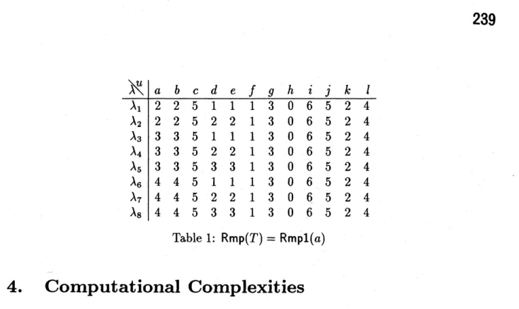
the computation ofmedian intervals. Let $T$ be an el-tree shown in Fig. 1 (i) and $T^{(a)}$ be

the tree $T$ rooted at node _$a$ (Fig. 2 $(i)$). Then we have the map $I$on $T^{(a)}$ (Fig. 2 (ii)) and

by using the depth first search on the set $V$ of nodes, each MPR $\lambda$ on _$T$ is defined and

shown in Table 1:

$\lambda(a)\in[2,4]$

A$(a)=2$

$\lambda(b)\in med\langle[2,2], [2,2], [4,4]\rangle=[2,2]$

$A(b)=2$

$\lambda(c)\in med\langle[2,2], [5,5], [6,6]\rangle=[5,5]$

$A(c)=5$

$\lambda(d)\in med\langle[2,2], [1,1], [0,3]\rangle=[1,2]$

$A(d)=1$

$\lambda(e)\in med\langle[1,1], [3,3], [0,0]\rangle=[1,1]$

$A(e)=1$

$A(d)$ : 2

$\lambda(e)\in med\langle[2,2], [3,3], [0,0]\rangle=[2,2]$

$A(e)=2$

Table 1: $Rmp(T)=Rmpl(a)$

4.

Computational Complexities

Onesees in the previous sectionsthat the description oftheproblem andthealgorithms

is simple but theproofofvalidity ofthe algorithms is not so simple. Thecomplexity analysis

is also not so difficult, because all the key concepts arerecursively defined.

First of all, considering the well-definability of $L^{*}(T)$ for a given el-tree $T$, which is

mentioned in Introduction, we see that it is sufficient for solving the MPR problem to

examine $\delta^{h}$ reconstructions on _$T$

,

where

$\Delta=[\min\sigma,\max\sigma],$ $\delta$ is the cardinality of $\Delta$ and

$h(=|V_{H}|)$ is the number of internal nodes of$T$

.

When $\Omega=N$, we could solve the MPR

problemby the primitive finite algorithn, i.e., the method of checking all posibihties, since

$\delta^{h}<\infty$, but the complexity order is exponential. When _$\Omega=R$, note that $\delta^{h}$ is not finite.

We now discuss about the algorithmic complexity of our algorithms for the following

four problems:

1. determine $L^{*}(T)$ for agiven el-tree $T$,

2. find any one MPR on a given el-tree,

3. enumerate all MPRs on a given el-tree.

We must appreciate that the description of the “sorted” sequence of end points of

closed intervals in $\Omega$ is often used in the previous sections, but the number ofcomparisons

required to “select” the i-th smallest of$n$ numbers (denoted by $f(i,$$n)$) is essential in the

complexity analysis ofour algorithms. Therefore,our timecomplexity analysis is basedon

the following result (Theorem 1 in p.450 of [1]) for the selection algorithm called PICK by

Blum et al. [1].

PICK Theorem. The number $f(i, n)$

of

comparisons required to select the i-th smallest

of

$n$ numbers is at most a linear

function of

$n,$ $i.e.,$ $f(i, n)=O(n)$

.

Theorem 2. The complexity

_of

our algorithm

_for

Problem 1 is $O(n)$

for

the number$n$

of

240

Theorem 3. The complexity

_of

our algorithm

_for

Pmblem

2

is $O(n)$

for

the number$n$

of

nodes in a given el-tree.

When $\Omega=R,$ $wedonotdiscussthecomplexityofalgorithmforProblem3bytheobvious$

reason.

Proposition 1.

When

$\Omega=N_{f}$ there is an el-tree $T$ such that the number

of

all MPRs on

$T$ is exponential

for

the number $n$

of

the nodes.

Proof. Consider the rooted el-tree $T^{(a)}$ shown in Fig. 3. $\square$

A tree with $10m+1$ modes and at least $5^{2m}$ MPRs.

Fig. 3.

References

[1] M. Blum, R. W. Floyd, V. Pratt, R. L. Rivest, and R. E. Tarjan, Time bounds for

selection, Journal ofComputer and System Sciences

7

(1973)

448-461.

[2] N. Minaka, Parsimony, phylogeny and discrete mathematics: combinatorial problems

in phylogenetic systematics (in Japanese: with English summary), Natural History

Research, Chiba Prefectural Museumand Institute, Vol.2 No.2 (1993) 83-98.

[3] D. L. Swofford and W. P. Maddison, Reconstructing ancestral character states under

Wagner parsimony, Mathematical Biosciences

87

(1987)

199-229.

[4] M. Hanazawa, H. Narushima and N. Minaka, Generating most parsimonious

recon-structions on a tree: a generalization of the Farris-Swofford-Maddison method, to

appear.

[5] M. Hanazawa and H. Narushima, A more efficient algorithmforMPR problems on an

el-tree, to appear.

[6] H. Narushima and N. Misheva, On the positions ofAcctran and Deltran in the