Bug prediction based on fine-grained module histories

全文

(1)奈良先端科学技術⼤学院⼤学学術リポジトリ Nara Institute of Science and Technology Academic Repository: naistar. Title. Bug prediction based on fine-grained module histories. Author(s). Hata, Hideaki ; Mizuno, Osamu; Kikuno, Tohru. Citation. ICSE 2012 : 2012 34th International Conference on Software Engineering, 2-9 June 2012, Zurich, Switzerland. Issue Date. 2012. Resource Version. author © 2012 IEEE. Personal use of this material is permitted. Permission from IEEE must be obtained for all other uses, in any current or future media,. Rights. including reprinting/republishing this material for advertising or promotional purposes, creating new collective works, for resale or redistribution to servers or lists, or reuse of any copyrighted component of this work in other works.. DOI. 10.1109/ICSE.2012.6227193. URL. http://hdl.handle.net/10061/12751.

(2) Bug Prediction Based on Fine-Grained Module Histories Hideaki Hata∗ , Osamu Mizuno† , and Tohru Kikuno∗ ∗ Osaka University, Osaka, Japan {h-hata, kikuno}@ist.osaka-u.ac.jp † Kyoto Institute of Technology, Kyoto, Japan o-mizuno@kit.ac.jp. Abstract—There have been many bug prediction models built with historical metrics, which are mined from version histories of software modules. Many studies have reported the effectiveness of these historical metrics. For prediction levels, most studies have targeted package and file levels. Prediction on a fine-grained level, which represents the method level, is required because there may be interesting results compared to coarse-grained (package and file levels) prediction. These results include good performance when considering quality assurance efforts, and new findings about the correlations between bugs and histories. However, fine-grained prediction has been a challenge because obtaining method histories from existing version control systems is a difficult problem. To tackle this problem, we have developed a fine-grained version control system for Java, Historage. With this system, we target Java software and conduct fine-grained prediction with wellknown historical metrics. The results indicate that fine-grained (method-level) prediction outperforms coarse-grained (package and file levels) prediction when taking the efforts necessary to find bugs into account. Using a correlation analysis, we show that past bug information does not contribute to method-level bug prediction. Keywords-bug prediction; fine-grained prediction; finegrained histories; historical metrics; effort-based evaluation. I. I NTRODUCTION Bug prediction has been widely studied and has been one of many hot topics among researchers. Recent findings show the usefulness of collecting historical metrics from software repositories for bug prediction models. Many studies measure software development histories, such as changes on source code [1], events of development or maintenance processes [2]–[5], developer-related histories [6]–[13], and so on. It is reported that historical metrics are more effective than code complexity metrics [14], [15]. In industry, there are reports of bug prediction in practice. Microsoft Corporation built a system, CRANE, and reported its experiences with this system [16]. Historical metrics including code churn, regression histories, and details of fixes are collected to build failure prediction models in CRANE. There is also a report of bug prediction in practice at Google1 . Based on research papers [4], [17], a prediction model was built using bug-fix information. In both industry and the academy, bug prediction with historical metrics has 1 Bug Prediction at Google, http://google-engtools.blogspot.com/2011/12/ bug-prediction-at-google.html. become the focus of attention because of its effectiveness and understandability. In the research area of bug prediction, fine-grained prediction is one of the next challenges. In the ESEC/FSE 2011 conference, PhD working groups created a forum to conduct short surveys on software engineering topics by interviewing conference participants and researching the field2 . The forum group who discussed “bug prediction models” concentrated on the main open challenges in building bug prediction models. From 27 subjects, including five from industry and 22 from academia, fine-grained prediction was selected as one of the future directions. Studies of fine-grained prediction are necessary because desirable results may be obtained when compared to coarse-grained prediction. Recently, studies take into account the effort of quality assurance activities for evaluating bug prediction results [17]–[21]. Effort-based evaluation considers the effort required to find bugs, but does not evaluate the prediction results only with prediction accuracy. Previous studies considered the lines of code (LOC) of modules as efforts. If we can find the most bugs while investigating the small percentages of LOC in the entire software, such prediction models would be desirable. Recent studies reported that file-level prediction models are more effective than package-level prediction, which has more coarse-grained modules than file-level, on Java software [15], [22], [23]. From these results, we can hypothesize that method-level prediction is more effective than package-level and file-level prediction, which means we can find more bugs during quality assurance activities with method-level prediction while investigating the same amount of LOC. Actually, there are studies predicting fine-grained buggy modules. Kim et al. targeted buggy Java methods by a cachebased approach [4]. Mizuno and Kikuno predicted buggy Java methods using a spam-filtering-based approach [24]. However, there have been few studies of fine-grained prediction using well-known historical metrics. This is because of the difficulty of collecting method-level historical metrics since version control systems do not control method histories. To collect detailed histories, we have proposed a finegrained version control system, Historage [25]. Historage is 2 http://pwg.sed.hu/.

(3) constructed on top of Git, and can control method histories of Java. With this system, we collect historical metrics for methods to build prediction models, and compare such models with package-level and file-level prediction models based on effort-based evaluation. We empirically evaluate the prediction models with eight open source projects written in Java. The contributions of this paper can be summarized as follows: • Survey and classification of recent historical metrics proposed in bug prediction studies. • Study of the effectiveness of method-level prediction compared with package-level and file-level prediction based on effort-based evaluation, and a report of its effectiveness. • Analysis of the correlations between bugs and histories of packages, files, and methods. The reminder of this paper is structured as follows. Section II summarizes the proposed historical metrics from our survey. Section III discusses the problem of obtaining finegrained module histories, and introduces our fine-grained version control system. In Section IV, we describe our study design, including effort-based evaluation, research questions, information of study projects, collected historical metrics in our study, and how we collect buggy modules, and the prediction model we used. Section V reports the results and lessons we learned, and Section VI discusses the overheads of fine-grained prediction and threats to the validity of this study. Finally, we conclude in Section VII. II. H ISTORICAL M ETRICS In this Section, we classify historical metrics based on the target of measurement. We prepare four categories each of code-related metrics, process-related metrics, organizational metrics, and geographical metrics. A. Code-Related Metrics Nagappan and Ball proposed code churn metrics, which measures the changes made to a module over a development history [1]. They measured Churned LOC / Total LOC, and Deleted LOC / Total LOC, for example. Churned LOC is the sum of added and changed lines of code between a baseline version and a new version of a module. Based on code churn metrics the authors built statistical regression models, and reported that code churn metrics are highly predictive of defect density performed on Windows Server 2003. These code-related metrics have been basic historical metrics and have been used in many studies [10], [14], [15], [26]–[30]. B. Process-Related Metrics There are many studies of historical metrics related to development processes. Changes, fixes, past bugs, etc. Graves et al. measured the number of changes, the number of past bugs, and the average. age of modules for predicting bugs [2]. They reported the usefulness of such process-related metrics compared with traditional complexity metrics from a telephone switching system study. These process-related metrics have been used in many studies, for example, the number of changes [3], [4], [6], [7], [9], [10], [14], [15], [30], [31] , the number of past bugs [27], [29], [31], [32], the number of bug fix changes [3], [4], [6], [14], [15], [30], [33], and module ages [3], [4], [6], [15], [26], [30], [31]. Cache-based approach. Several cache-based bug prediction studies exist [3], [4], [17]. Hassan and Holt, for example, proposed a “Top Ten List,” which dynamically updated the list of the ten most likely subsystems to have bugs [3]. The list is updated based on heuristics including the most recently changed, most frequently bug fixed, and the most recently bug fixed as the development progresses. Kim et al. [4] and Rahman et al. [17] discusses BugCache and FixCache cache operations. The four heuristics used as cache update policies in their work are as follows: •. •. •. •. Changed locality: recently changed modules tend to be buggy. New locality: recently created modules tend to be buggy. Temporal locality: recently bug fixed modules tend to be buggy. Spatial locality: a module recently co-changed with bug-introduced modules tends to be buggy.. The number of co-changes with buggy modules (logical coupling with bug-introducing modules) are also measured in other studies [8], [14]. Process complexity metrics. Hassan proposed complexity metrics of code changes [5]. These metrics are designed to measure the complexity of change processes based on the conjecture that a chaotic change process is a good indicator of many project problems. The key idea is that the modules that are modified during periods of high change complexity will have a higher tendency to contain bugs. To measure the change complexity of a certain period, Hassan proposed to use Shannon’s Entropy. To measure how much a module is modified in complex change periods, different parameters are prepared and four history complexity metrics (HCM) are proposed. It is reported from a study with open source projects that history complexity metrics are better predictors than process-related metrics, i.e., prior modifications and prior bugs [5]. C. Organizational Metrics Historical metrics related to organization are newer metrics and have been well studied recently. Number of developers. Graves et al. measured the number of developers [2]. From a case study of a telephone switching system, the authors reported that the number of developers did not help in predicting the number of bugs..

(4) Weyuker et al. also reported that the number of developers is not a major influence on bug prediction models [6]. Structure of organization. To investigate a corollary of Conway’s Law, “structure of software system closely matches its organization’s communication structure” [34], Nagappan et al. designed organizational metrics, which include the number of engineers, the number of ex-engineers, the number of changes, the depth of master ownership, the percentage of organizational contribution, the level of organizational ownership, overall organizational ownership, and the organization’s intersection factor [7]. They reported that these organizational metrics-based failure-prone module prediction models achieved higher precision and recall values compared with models with churn, complexity, coverage, dependencies, and pre-release bug measures from a case study of Windows Vista. Mockus investigated the relationship between developercentric metrics of organizational volatility and the probability of customer-reported defects [8]. From a case study of a switching software project, Mockus reported that the number of developers leaving and the size of the organization have an effect on software quality, but the number of newcomers to the organization is not statistically significant. Network metrics. Networks between developers and modules are analyzed for predicting failures [9]–[11]. Human factors, such as the contributions of developers, coordination, and communications are examined based on network metrics, such as centrality, connectivity, and structural holes. Ownership. The relationship between ownership and quality is also investigated. Bird et al. examined the effects of ownership on Windows Vista and Windows 7 [12]. They measured the number of minor contributors, the number of major contributors, the total number of contributors, and the proportion of ownership for the contributor with the highest proportion of ownership. They found a high ratio of ownership and many major contributors, and a few minor contributors are associated with less defects. Rahman and Devanbu examined the effects of ownership and experience on quality [13]. They conducted a finegrained study about authorship and ownership of code fragments. They measured the number of lines contributed by an author divided by the number of lines changed to fix a bug as an authorship metric, and defined the authorship of the highest contributor as ownership. From a study of open-source projects, they reported that a high ownership value by a single author is associated with lines changed or deleted to fix bugs, and that lack of specialized experience on a particular file is associated with such lines. D. Geographical Metrics Geographical metrics are measured for assessing the risks of distributed development. Bird et al. investigated the locations of engineers who developed binaries [35]. Bird et al. classified distribution levels into buildings, cafeterias,. campuses, localities, and continents. From a case study of Windows Vista, they clarified how distributed development has little to no effect on post-release failures. In a study of organizational volatility and its effects on software defects, Mockus measured the number of sites that modified the file and investigated the distribution of mentors and developers [8]. He also reported on a case study of large switching software to show that geographic distribution has a negative impact on software quality. III. F INE -G RAINED H ISTORIES In Section II, we discussed various historical metrics. To measure these historical metrics, we need to obtain version histories of each module. For packages and files, it is easy to collect historical metrics by using builtin commands of ordinary version control systems. However, there is no command to investigate the histories of methods in Java files. To analyze fine-grained module histories, some tools have been proposed and used in research. Hassan and Holt, for example, proposed C-REX, which is an evolutionary extractor [36]. It records fine-grained entity changes over the development period. Although C-REX stores entire versions, it cannot track module histories if there is renaming or moving. BEAGLE is a research platform [37]. Using origin analysis, it can identify rename, move, split, and merge. However, the BEAGLE targets selected release revisions to apply origin analysis. Bevan et al. proposed Kenyon, which is designed to facilitate software evolution research [38]. Although Kenyon records entire versions, rename and move are not identified. Zimmermann proposed APFEL, which collects fine-grained changes in relational databases [39]. Although versions are stored entirely, APFEL does not identify rename or move. For fine-grained module histories, clarifying existing methods in particular revisions is not difficult because all versions of the files are stored entirely. Matching every sequential version is required to obtain entire method histories, but matching is difficult when renaming and moving exist. Because of this limitation, obtaining entire histories of Java methods has been difficult. To address this problem, we proposed a fine-grained version control system, Historage [25]. We make use of the rename/move detection mechanism of Git, a version control system. When renaming and moving exists, Git identifies matches based on the similarities of file contents. Historage stores all Java methods independently, and control their histories3 . Since Historage is created on top of a Git version control system, every Git command can be used. From empirical evaluation with some open source projects, we found that Historage can identify matches practically 3 A tool to create Historage is available from https://github.com/hdrky/ git2historage.

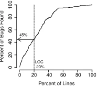
(5) 80 100 60 40. 45%. 20. B. Research Questions LOC 20%. 0. Percent of Bugs Found. this cutoff line, it is better for the cost of inspection and testing. In this example, when we inspect top bug-prone modules until 20% of the entire LOC, it is revealed that we can investigate 45% of buggy modules.. 0. 20. 40. 60. 80. 100. Percent of Lines. Figure 1.. Cost-effectiveness curve. when renaming and moving exist4 . With this system, we can obtain the entire histories of Java methods, and collect method-level historical metrics. IV. S TUDY D ESIGN A. Effort-Based Evaluation Recent studies take into account the effort of quality assurance activities, such as inspecting and testing predicted modules for evaluating prediction models [17]–[21]. These effort-based evaluations should be desirable for practical use of the prediction results. The key idea of effort-based evaluation is that it discriminates the cost of inspecting and testing for each module. Arisholm et al. pointed out that the cost of such quality assurance activities on a module is roughly proportional to the size of the module [20]. Figure 1 illustrates an example of a cost-effectiveness curve. This curve shows that as the quality assurance cost increases, the percentage of found bugs increases. The quality assurance cost is represented as the percentage of investigated LOC of software. When we inspect or test modules, the modules are ordered by bug-proneness. If we find most bugs when we investigate the small percentage of the entire LOC, it should be effective. To compare different bug prediction results, the percentage values of bugs found on the same value of the percentage of LOC should be easy to understand. For this cutoff value, 20% of LOC is used in some studies [15], [17], [20], [21]. We also choose 20% as this cutoff value because it is more realistic than investigating the entire LOC. Inspecting 20% of the entire LOC may be an enormous effort for large software, or little for small software. So deciding cutoff with absolute value of cumulative LOC is another possible way, and one of future works is to discuss the results with such effort-based evaluation. In Figure 1, a dotted line represents this cutoff of LOC at 20%. If cost-effectiveness curves cross the upper part of 4 Git detects rename/move while outputting logs with -M option if the content is similar enough. The default value of this similarity threshold is 50%. Historage makes use of this mechanism for tracking methods and we found that it detected more than 99% correct matches in candidates with this default threshold value.. To investigate the effectiveness of fine-grained prediction, we compare prediction models on different levels, that is, packages, files and methods of Java software. Prediction models are built with well-known historical metrics proposed and used in previous studies, and are compared with effort-based evaluation. Compared with package-level and file-level prediction, there is a difference in method-level prediction. Since packages consist of files, the total LOC are equal in both levels. However, this does not hold in package-level vs. methodlevel and file-level vs. method-level because a file does not consist of methods only. For fair comparison with levels of package, file, and method, we ignore code except for methods. This means that bugs only in methods are targeted, and only the LOC of methods are considered as efforts. With these settings, we investigate the following three research questions: RQ1: Are method-level prediction models more effective than package-level and file-level prediction models with effort-based evaluation? RQ2: (When method-level prediction models are more effective.) Why are method-level prediction models more effective than package-level and file-level prediction models? RQ3: Are there differences in different module levels regarding the correlations between bugs and module histories? C. Target Projects We selected eight open-source projects for our study: Eclipse Communication Framework (ECF), WTP Incubator, and Xpand were chosen from the Eclipse Projects. Ant, Cassandra, Lucene/Solr, OpenJPA, and Wicket were chosen from the Apache Software Foundation. All projects are written in Java and have relatively long development histories. We chose these projects because they span varied application domains: a building tool, a distributed database management system, a text search platform, an objectrelational mapping tool, a web application framework, and development platform plugins related to the communication framework, web tools, and a template engine. We obtained each Git repository5. For package-level and file-level prediction, we mine ordinary Git repositories. For method-level prediction, we convert ordinary Git repositories to Historage repositories, and mine them. This conversion 5 Eclipse Projects from http://git.eclipse.org/ and Apache Software Foundation from http://git.apache.org/.

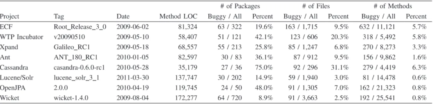
(6) Table I S UMMARY OF STUDIED PROJECTS Name. Initial Date. Last Date. # of Commits. # of Developers. Last LOC. # of Files on Last Date. ECF WTP Incubator Xpand Ant Cassandra Lucene/Solr OpenJPA Wicket. 2004-12-03 2007-11-10 2007-12-07 2000-01-13 2009-03-02 2010-03-17 2006-05-02 2004-09-21. 2011-05-31 2010-07-22 2011-05-31 2011-08-19 2011-09-20 2011-09-20 2011-09-15 2011-09-20. 9,748 1,133 1,038 12,590 4,423 3,485 4,180 15,033. 23 17 21 46 14 27 26 25. 167,283 206,533 79,589 118,969 99,940 347,898 343,191 410,538. 2,439 1,944 1,126 1,194 712 3,301 4,229 6,681. can be done automatically. Table I summarizes information for each target project. The development period ranges from 18 months to 11 years, and the LOC on the last date of the studied period ranges from 15k to 370k. Table I also presents the number of commits (from 1k to 15k), the number of developers (from 14 to 46), and the number of files on the last date (from 700 to 4k). The average LOCs per one file varies from 61.4 to 140.4. D. Metrics Collection We collected the major metrics discussed in Section II. Historical metrics for packages can be measured by the cumulating values of files in the packages in most cases. Method-level historical metrics can be collected from Historage repositories similar to collecting file-level historical metrics from Git repositories. Table II presents all historical metrics collected in this study. Code-related metrics. For code-related metrics, we measure LOC and code churn metrics (Added LOC and Deleted LOC). As stated in Section II-A, these metrics are used in many studies. Code churn metrics for files are easily collected from version control repositories. Process-related metrics. For process-related metrics, we collect the basic metrics stated in Section II-B, such as the number of changes, the number of past bugs, the number of bug-fix changes, and the existing period (age) of modules. Some metrics are collected inspired by cache-based approaches [3], [4], [17]. We collect two types of logical coupling metrics: the number of logical couplings with bugintroduced modules and the number of logical couplings with modules that have been buggy. To investigate the frequency of changes, we measured average, maximum, and minimum intervals. In addition, we also collected one of the history complexity metrics [5]. As stated in Section II-B, there are four types of historical complexity metrics. In this paper, we select HCM 3s because it performed well. This metric is designed under the assumption that modules are equally affected by the complexity of a period. For other parameters, we follow the paper [5].. Organizational metrics. Organizational metrics and geographical metrics are relatively difficult to collect from opensource projects although it may be possible to measure by integrating information from several software repositories. Hence, we measure ownership-related metrics designed in [12] although there are lots of metrics, especially for organizational metrics as stated in Section II-C. Organizational metrics in [12] can be collected only from version control repositories. To measure ownership-related metrics, we follow the definition of proportion of ownership in [12]. The proportion of ownership of a developer for a particular module is the ratio of the number of changes by the developer to the number of total changes for that module. If ownership of an developer is below a threshold, the developer is considered a minor developer, otherwise, a major developer. In [12], values ranging from 2% to 10% are suggested as the threshold based on a sensitivity analysis. Bird et al. targeted compiled binaries as modules for study, which tend to be developed by many developers [12]. On the contrary, files and methods, which are our modules for study, are a relatively small size and are developed by relatively only a few developers. To take into account this difference, we set the threshold value at 20%. E. Bug Information Buggy modules are collected based on the SZZ algorithm ´ (proposed by Sliwerski, Zimmermann, and Zeller), which is designed to identify bug-introducing commits by mining version control repositories and bug report repositories [40]. Buggy modules can be identified by choosing modified modules between bug-introducing commits and bug-fixing commits. With the SZZ algorithm, bug-introducing and bugfixing commits can be linked with each bug ID in bug reports6 . First, we need bug reports from bug report repositories, such as Bugzilla and JIRA. In these bug report repositories, 6 Bug reports are available from https://bugs.eclipse.org/bugs/ (Eclipse Projects), https://issues.apache.org/bugzilla/ (Ant), and https://issues. apache.org/jira/ (the other projects in the Apache Software Foundation).

(7) Table II C OLLECTED HISTORICAL METRICS Name. Description. Code. LOC AddLOC DelLOC. Lines of code Added lines of code from the initial version Deleted lines of code from the initial version. Process. ChgNum FixChgNum PastBugNum Period BugIntroNum LogCoupNum AvgInterval MaxInterval MinInterval HCM. Number of changes Number of bug-fix changes Number of fixed bug IDs Existing period in days Number of logical coupling commits that introduce more than one bug in other modules Number of logical coupling commits that change other modules that have been buggy Period /ComNum Maximum weeks between two sequential changes Minimum weeks between two sequential changes History complexity metric HCM 3s. Organization. DevTotal DevMinor DevMajor Ownership. Total number of developers Number of minor developers Number of major developers The highest proportion of ownership Table III S UMMARY OF PREDICTION MODULES. Project. Tag. Date. ECF WTP Incubator Xpand Ant Cassandra Lucene/Solr OpenJPA Wicket. Root Release 3 0 v20090510 Galileo RC1 ANT 180 RC1 casandra-0.6.0-rc1 lucene solr 3 1 2.0.0 wicket-1.4.0. 2009-06-02 2009-05-10 2009-05-18 2010-01-05 2010-05-28 2011-03-30 2010-04-19 2009-08-04. Method LOC 81,324 58,407 68,557 82,597 35,179 137,747 119,745 172,277. there are also reports for requesting new features or enhancement. To ignore such reports, it is necessary to filter reports. From Bugzilla repositories, we exclude enhancement severity reports, and from JIRA repositories, we collect only bug issue type reports. From a bug report of bug bi , where i represents bug ID, we obtain open date OD(bi ) and commit date CD(bi ). With collected bug reports, we then identify bug-fixing commits. Bug-fixing commits and bug bi are linked based on matching bug IDs in commit messages stored in version control repositories. While linking commits and bug bi , we investigated whether commit dates are before CD(bi ) or not to remove improper identification of bug-fixing commits. From each bug-fixing commit, we perform the following procedure to identify buggy modules: 1) Perform the ‘diff’ command on the same module between the bug-fixing version and a preceding revision to locate modified regions on the bug-fixing commit.. # of Packages Buggy / All Percent 63 / 322 51 / 121 55 / 213 30 / 83 27 / 36 30 / 202 24 / 50 64 / 720. 19.6% 42.1% 25.8% 36.1% 75.0% 14.9% 48.0% 8.9%. # of Files Buggy / All Percent 163 / 1,715 123 / 606 85 / 1,247 87 / 912 92 / 296 59 / 1,940 91 / 1,305 91 / 3,663. 9.5% 20.3% 6.8% 9.5% 31.1% 3.0% 7.0% 2.5%. # of Methods Buggy / All Percent 632 / 11,121 318 / 5,492 270 / 8,273 156 / 9,862 279 / 4,419 81 / 14,478 162 / 21,323 192 / 25,541. 5.7% 5.8% 3.3% 1.6% 6.3% 0.6% 0.8% 0.8%. 2) Examine the initially inserted date of the modified regions using line tracking commands, such as ‘git blame’ or ‘cvs annotate’. If the regions are inserted before OD(fi ), commits creating those regions are identified as bug-introducing commits. 3) Identify a module as buggy if the module contains regions that are created in the bug-introducing commits, and are modified in the bug-fixing commits. As reported in [41], naive differencing analysis on step 1 of the procedure should yield incorrect bug-introducing commits, such as non-behavior change commits and just format change commits. To remove such false positives, we ignore changes on blank lines, comment changes, and format changes. In addition, we ignore changes not on methods to identify bugs on methods as stated in Section IV-B. This procedure can be performed automatically. If there is more than or equal to one buggy file in a package, we consider it as a buggy package. Buggy methods are identified by.

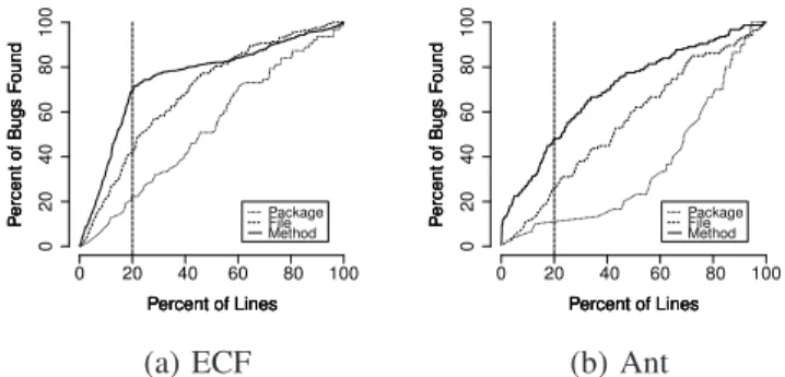
(8) V. R ESULTS We present our results following research questions stated in Section IV-B. Plots of the results are shown from Eclipse Communication Framework (ECF) and Ant only, and other results are discussed in text.. 80 100 60 40 20. Percent of Bugs Found. 80 100 60 40 20. Package File Method. 0. Percent of Bugs Found. 0. 20. 40. 60. 80. 100. 0. 20. 40. 60. 80. Percent of Lines. Percent of Lines. (a) ECF. (b) Ant. 100. 40 0. 20. 40. 60. Percent of Bugs Found. 60. 80. Figure 2. Cost-effectiveness curves of package-level, file-level and methodlevel prediction. 20. Bug prediction models are built with the historical metrics shown in Section IV-D. These historical metrics are measured in the period from the initial date to the tagged date shown in Table III for each module. We adopt the RandomForest algorithm [42] as a bug prediction model. RandomForest is a classifier with many decision trees that outputs the class that is the mode of the classes output by individual trees. Lessmann et al. confirmed its good performance in bug prediction [43]. There are several other studies using the RandomForest algorithm for bug prediction [15], [21]. We use a statistical computing and graphics tool R [44] and a randomForest package for our study. As shown in Table III, the percentages of buggy methods are small in total methods. In such cases, prediction models tend to predict all methods as non-buggy because there are only a small number of false positives. In our pilot study with other prediction models like logistic regression, we found such results. However, with RandomForest models, not all methods are predicted as non-buggy in every project. Using prepared modules in Table III, we conduct a 10-fold cross validation analysis. Entire modules in one prediction level in one project are randomly divided into 10 groups. Of the 10 groups, a single group is used for testing a model, and the other 9 groups are used for training the model. The cross-validation process is repeated 10 times, with each of the 10 groups used once as test data. The 10 results are combined into a single validation result.. 0. Percent of Bugs Found. F. Prediction Model. Package File Method. 0. mining Historage repositories. This identification can also be performed automatically. We identify buggy packages, files, and methods in one revision for each project. For this particular revision, we select tagged revisions or revisions that are nearby tagged revisions. Table III shows the data of the prediction study and the result of buggy module identification. We obtained bug reports from the first report to the last one until June 30, 2011. With these reports and entire versions in obtained version repositories, we identify bug information. The percentages of buggy packages ranges from 8.9% to 75.0%, the percentages of buggy files ranges from 2.5% to 31.1%, and the percentage of buggy methods ranges from 0.6% to 6.3%. Since we target only the code of methods, each total LOC is accumulated with the entire method LOC (Method LOC).. Package. File. (a) ECF. Method. Package. File. Method. (b) Ant. Figure 3. Boxplots of package-level, file-level, and method-level prediction. Percentages of bugs found in 20% LOC on a 1, 000 times run. A. Effort-Based Evaluation: Package, File vs. Method RQ1: Are method-level prediction models more effective than package-level and file-level prediction models with effort-based evaluation? Figure 2 shows two plots of cost-effectiveness curves. A package-level curve (dotted), file-level curve (dashed), and a method-level curve (solid) are plotted. We can see that the method-level curves rise larger than the packagelevel and file-level curves in a small LOC. As a result, more bugs can be found by method-level prediction when investigating 20% of the LOC, represented by the cutoff lines. In all projects, method-level prediction outperformed package-level and file-level prediction. As Arcuri and Briand insisted, we should collect data from a large enough number of runs to assess the results of randomized algorithms because we obtain different results on every run when applied to the same problem instance [45]. RandomForest is a randomized algorithm. Figure 2 shows the result on one run. Following the suggested value of 1, 000 as a very large sample [45], we conducted a 1, 000 times run for all projects. Figure 3 shows the results of the 1, 000 run. In each project, boxplots of the value of percentages of bugs found in 20% LOC for package-level, file-level and method-level are shown. In all projects, we observed the small distributions.

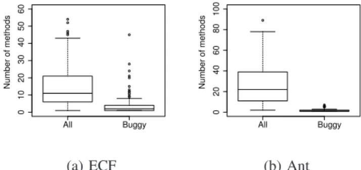
(9) B. Why Is Method-Level Prediction Effective? RQ2: Why are method-level prediction models more effective than package-level and file-level prediction models? Intuitively, fine-grained prediction may more effective than coarse-grained prediction because finding bugs in large modules is difficult. Figure 4 shows boxplots of LOC for packages, files, and methods. With the Mann-Whitney Utest in all pairwise comparisons (packages vs. files, packages. 1500 1000. LOC. 500. 400. 0 Package. File. Method. Package. (a) ECF. Method. (b) Ant. 60 40. Number of methods. 80 100. Size of modules: package-level, file-level and method-level.. 20. Figure 4.. File. 0. of the values, and method-level prediction achieved higher values than package-level and file-level prediction. In Table IV, we summarize the median values of the percentages of found bugs when investigating 20% of LOC in all modules. The second to fourth column shows the values of package-level, file-level, and method-level results. To detect statistical differences, the Mann-Whitney U-test was used between package-level vs. method-level and filelevel vs. method-level. In both pairs in all projects, the differences are statistically significant (p < 0.001). The values of the percentages of found bugs are shown in bold if the value is more than 40%. In all projects, method-level prediction achieved more than 40%, and outperformed package-level and file-level prediction. Based on these results from eight open-source projects, we can answer research question RQ1. The answer is clear: method-level prediction is more effective than both package-level and filelevel prediction. When comparing package-level and file-level, file-level prediction outperformed package-level prediction in five projects as shown in Table IV. These results are consistent with the reports of previous studies [15], [22], [23]. However, there are opposite results in the Xpand, Cassandra, and OpenJPA projects. Our study is different from the previous studies in counting LOC and targeting bugs: we limit the LOC of methods and target buggy methods. These settings lead to an ignorance of files that have no method, and may improve the package-level prediction. However, these results depend on project-specific data. Therefore, analyzing these project-specific features is remained as a future work.. 200. 69.2 61.0 51.9 44.9 46.6 59.3 45.1 82.3. 0. Method. 42.3 37.4 12.9 25.3 20.7 52.5 16.5 65.9. 30 40 50 60. File. 19.1 29.4 35.2 13.3 22.2 17.2 20.8 60.9. Number of methods. Package. 10 20. ECF WTP Incubator Xpand Ant Cassandra Lucene/Solr OpenJPA Wicket. 0. Project. LOC. 600. 800. Table IV M EDIAN VALUES OF THE PERCENTAGE OF BUGS FOUND IN 20% LOC ON 1, 000 TIMES RUN. All. Buggy. (a) ECF Figure 5.. All. Buggy. (b) Ant. Number of all and buggy methods in buggy files.. vs. methods, and files vs. methods), we found that the differences in LOC are statistically significant (p < 0.001). Comparing the median value of the LOC, methods are nearly ten times smaller than files, and are from thirty to threehundreds times smaller than packages. Next, we investigated buggy files by considering how many methods exist in one file, and how many buggy methods exist in the file. The boxplots of Figure 5 present the results. In both projects, most of the buggy files contain nearly or more than 10 methods, but there are only a few buggy methods. From all of the projects, the median values of the number of entire methods range from 8 to22, and the median values of the number of buggy methods range from 1 to 2. Although there are many methods in one buggy file, there are only a few actual buggy methods. This indicates that we need to investigate most of the non-buggy methods in a file if the file is predicted to be buggy. Similarly, we also investigated buggy packages. From all of the projects, the median values of the number of entire methods range from 27 to 579.5, and the median values of the number of buggy methods range from 1 to 5.5. Because of these non-buggy methods, method-level prediction is more effective than package-level and file-level prediction..

(10) Table V S PEARMAN CORRELATION BETWEEN THE POST BUGS AND COLLECTED METRICS . M ARKED BY * IF STATISTICALLY SIGNIFICANT (p < 0.05). Metric. Package. ECF File. Method. Package. Xpand File. Method. Package. Ant File. Method. Package. Wicket File. Method. LOC AddLOC DelLOC ChgNum FixChgNum PastBugNum Period BugIntroNum LogCoupNum AvgInterval MaxInterval MinInterval HCM DevTotal DevMinor DevMajor Ownership. 0.392* 0.374* 0.259* 0.268* 0.333* 0.325* 0.139* 0.307* 0.312* -0.229* -0.108 -0.120* 0.249* 0.198* 0.225* 0.014 -0.105. 0.366* 0.063* 0.069* 0.017 0.138* 0.137* 0.146* 0.199* 0.163* 0.059* 0.084* 0.095* 0.200* 0.027 0.101* -0.040 -0.010. 0.239* 0.003 0.006 -0.007 0.044* 0.044* 0.129* 0.080* 0.089* 0.109* 0.121* 0.114* 0.142* -0.024* -0.010 -0.023* 0.024*. 0.303* 0.416* 0.416* 0.406* 0.299* 0.334* 0.316* 0.126 0.331* -0.372* -0.329* -0.295* 0.325* 0.571* 0.381* 0.463* -0.547*. 0.298* 0.237* 0.206* 0.212* 0.169* 0.170* 0.196* 0.228* 0.146* -0.126* -0.033 -0.138* 0.204* 0.259* 0.091* 0.262* -0.256*. 0.205* 0.213* 0.210* 0.192* 0.051* 0.051* 0.153* 0.161* 0.139* -0.035* -0.021 -0.035* 0.174* 0.234* -0.004 0.234* -0.236*. 0.493* 0.515* 0.366* 0.583* 0.550* 0.565* 0.302* 0.508* 0.429* -0.587* -0.606* -0.245* 0.564* 0.580* 0.566* -0.024 -0.431*. 0.362* 0.319* 0.246* 0.302* 0.331* 0.329* 0.139* 0.278* 0.202* -0.310* -0.297* -0.212* 0.257* 0.290* 0.305* -0.063 -0.178*. 0.164* 0.114* 0.098* 0.112* 0.096* 0.096* -0.001 0.088* 0.040* -0.113* -0.086* -0.105* 0.060* 0.101* 0.137* 0.039* -0.082*. 0.154* 0.181* 0.075* 0.126* 0.337* 0.339* -0.389* 0.223* 0.288* -0.261* -0.450* -0.108* -0.210* -0.099* 0.118* -0.016 -0.001. 0.159* 0.089* 0.095* 0.083* 0.199* 0.200* -0.207* 0.160* 0.144* -0.178* -0.230* -0.093* -0.095* 0.067* 0.065* 0.045* -0.049*. 0.094* 0.072* 0.067* 0.073* 0.098* 0.099* -0.104* 0.069* 0.053* -0.110* -0.118* -0.090* -0.055* 0.070* 0.022* 0.069* -0.068*. C. Correlation Analysis RQ3: Are there differences in different module levels regarding the correlations between bugs and module histories? The Spearman correlation values between historical metrics and the number of post bugs for package-level, file-level, and method-level of four projects are shown in TableV. The number of post bugs is the number of bug IDs that have not been fixed. Correlations that are statistically significant (p < 0.05) are marked by *. As shown in Table III, the percentages of buggy methods is smaller than the percentages of buggy packages and files. Thus the correlation values are lower in method-level. We can make the following observations: •. •. •. Code-related metrics have relatively higher correlations; that is, changes in code are related to bugs. Although this holds in most projects, there are exceptional projects like the Wicket project. In this project, Java files and methods do not change repeatedly. The usefulness of code-related metrics depends on how the software has evolved. Past bug information (FixChgNum and PastBugNum) does not correlate with post bugs for method-level prediction. This indicates that methods do not have bugs repeatedly. Metrics about intervals have negative correlations. In other words, short intervals between changes are related to bugs in most projects.. •. Organizational metrics may not contribute to methodlevel prediction. This is because many developers have not changed the methods in the studied projects.. VI. D ISCUSSION A. Overheads For method-level prediction, we need additional costs for package-level and file-level prediction. Required overheads can be summarized as follows: 1) Preparing Historage: Converting Git repositories to Historage repositories is needed only for method-level prediction. Although it takes several hours (a one night run), there is no need for manual efforts. 2) Mining Historage: Running the SZZ algorithm to identify buggy modules and collecting historical metrics require mining repositories of version control systems. The essential differences between Git repositories and Historage repositories is the number of storing modules. To calculate the LOC of one module, there is no difference in processing time. When we extract a single entire module’s history, rename/move identification requires an O(n2 ) processing time where n is the number of candidates. As a result, to mine a single log to collect simple historical metrics, such as the number of changes, fixes, and developers, Historage requires more processing time than Git. To collect the process complexity metrics, Historage requires more processing time because it needs to analyze multiple logs. 3) Building Models and Prediction: The processing time of training and testing models highly depends.

(11) on the number of modules. Actually, the most timeconsuming task in this study is the 1, 000 times run of 10-fold cross validation analysis for method-level prediction (it requires one to two days). Although there are such overheads, we do not need additional manual procedures for method-level prediction compared with package-level and file-level prediction. So we do not consider them as critical limitations. B. Threats to Validity Target projects are limited to open-source software written in Java. For external validity, there is a threat of generalization of our result. Projects we targeted are only open-source projects written in Java. One of the good points of targeting only open-source software projects in Java is that there is no opposite result regarding the effectiveness of method-level prediction compared with package-level and file-level prediction. As described in Section IV-C, the eight targeted projects varied in sizes, domains, and development periods. For example, the Lucene/Solr project has less than two periods, and prediction is conducted with only a one-year history and yields a good result. This result may promote the adoption of historical metrics based prediction for young projects. For future work we intend to widen our study to other projects written in other programming languages, and work on industrial projects. Collection of bug information has problems. For construct validity, the main threat is in the phase of collecting bug information. Although we adopted a well-known SZZ algorithm discussed in Section IV-E, it has been reported that there is a linking bias in identifying bugs with revision logs and bug reports [46]. Recently, a new algorithm of linking bugs and changes has been proposed [47]. This algorithm may mitigate this threat. Effort-based evaluation may not reflect actual efforts. In our evaluation, there are also threats to construct validity. To compare package-level, file-level, and methodlevel prediction, we adopted an effort-based evaluation with cost-effectiveness curves, which has been previously studied [17]–[21]. This effort-based evaluation considers the cost of quality assurance activities to be roughly proportional to the size of the modules, that is, to the lines of code. For coarse-grained modules, such as packages and files, it seems acceptable to consider the sizes of the modules as effort. However, for methods, it may not be acceptable. For example, although methods are small, they might require much more effort than big methods because of the context of the methods, such as complex call relations or other deep dependencies. Discussing these threats is also important for further finegrained prediction. When we consider only the sizes of the modules as efforts, we can hypothesize that blocklevel or line-level prediction is more effective than method-. level prediction for finding bugs. However, this hypothesize should not be acceptable. Because of this threat, we need empirical studies of the actual effort, such as times needed, and cumulative LOC of the code we need to inspect, by conducting actual quality assurance activities with different prediction levels. VII. C ONCLUSION This paper conducted fine-grained bug prediction, which is a method-level prediction, on Java software based on recently proposed historical metrics. Using eight open source projects, package-level, file-level, and method-level prediction models were compared based on effort-based evaluation. The findings from our study are as follows. Method-level prediction is more effective than package-level and filelevel prediction when considering efforts. This is because predicted buggy packages and files contain many non-buggy packages and files. From the correlation analysis, we found that past bug information on methods does not correlate with post bugs in methods, and organizational metrics may not contribute to method-level prediction. Code-related metrics have positive correlations and interval-related metrics have negative correlations. Effort-based evaluation may not reflect actual efforts. Therefore, in the future we will also use well-designed effort calculation or an empirical study of the actual efforts should be required. Correlation analysis is also needed for further study. To discuss the correlations between post bugs and historical metrics, we need more various-type projects to study. In addition, we want to compare fine-grained historical metrics with complexity metrics on methods. ACKNOWLEDGMENT This research is supported by a Grant-in-Aid for JSPS Fellows (No.23-4335) and a Grant-in-Aid for Scientific Research (c) (21500035) Japan. R EFERENCES [1] N. Nagappan and T. Ball, “Use of relative code churn measures to predict system defect density,” In ICSE ’05, pp. 284–292, 2005. [2] T. L. Graves, A. F. Karr, J. S. Marron, and H. Siy, “Predicting fault incidence using software change history,” IEEE Trans. Softw. Eng., vol. 26, pp. 653–661, July 2000. [3] A. E. Hassan and R. C. Holt, “The top ten list: Dynamic fault prediction,” In ICSM ’05, pp. 263–272, 2005. [4] S. Kim, T. Zimmermann, E. J. Whitehead Jr., and A. Zeller, “Predicting faults from cached history,” In ICSE ’07, pp. 489–498, 2007. [5] A. E. Hassan, “Predicting faults using the complexity of code changes,” In ICSE ’09, pp. 78–88, 2009. [6] E. J. Weyuker, T. J. Ostrand, and R. M. Bell, “Do too many cooks spoil the broth? using the number of developers to enhance defect prediction models,” Empirical Softw. Eng., vol. 13, pp. 539–559, October 2008. [7] N. Nagappan, B. Murphy, and V. Basili, “The influence of organizational structure on software quality: an empirical case study,” In ICSE ’08, pp. 521–530, 2008..

(12) [8] A. Mockus, “Organizational volatility and its effects on software defects,” In FSE ’10, pp. 117–126, 2010. [9] M. Pinzger, N. Nagappan, and B. Murphy, “Can developermodule networks predict failures?” In SIGSOFT ’08/FSE-16, pp. 2–12, 2008. [10] A. Meneely, L. Williams, W. Snipes, and J. Osborne, “Predicting failures with developer networks and social network analysis,” In SIGSOFT ’08/FSE-16, pp. 13–23, 2008. [11] T. Wolf, A. Schroter, D. Damian, and T. Nguyen, “Predicting build failures using social network analysis on developer communication,” In ICSE ’09, pp. 1–11, 2009. [12] C. Bird, N. Nagappan, B. Murphy, H. Gall, and P. Devanbu, “Don’t touch my code!: examining the effects of ownership on software quality,” In ESEC/FSE ’11, pp. 4–14, 2011. [13] F. Rahman and P. Devanbu, “Ownership, experience and defects: a fine-grained study of authorship,” In ICSE ’11, pp. 491–500, 2011. [14] R. Moser, W. Pedrycz, and G. Succi, “A comparative analysis of the efficiency of change metrics and static code attributes for defect prediction,” In ICSE ’08, pp. 181–190, 2008. [15] Y. Kamei, S. Matsumoto, A. Monden, K. Matsumoto, B. Adams, and A. E. Hassan, “Revisiting common bug prediction findings using effort-aware models,” In ICSM ’10, pp. 1–10, 2010. [16] J. Czerwonka, R. Das, N. Nagappan, A. Tarvo, and A. Teterev, “CRANE: Failure prediction, change analysis and test prioritization in practice – experiences from windows,” In ICST ’11, pp. 357–366. [17] F. Rahman, D. Posnett, A. Hindle, E. Barr, and P. Devanbu, “BugCache for inspections: hit or miss?” In ESEC/FSE ’11, pp. 322–331, 2011. [18] A. G. Koru, K. E. Emam, D. Zhang, H. Liu, and D. Mathew, “Theory of relative defect proneness,” Empirical Softw. Eng., vol. 13, pp. 473–498, October 2008. [19] T. Menzies, Z. Milton, B. Turhan, B. Cukic, Y. Jiang, and A. Bener, “Defect prediction from static code features: current results, limitations, new approaches,” Automated Softw. Eng., vol. 17, pp. 375–407, December 2010. [20] E. Arisholm, L. C. Briand, and E. B. Johannessen, “A systematic and comprehensive investigation of methods to build and evaluate fault prediction models,” J. Syst. Softw., vol. 83, pp. 2–17, January 2010. [21] T. Mende and R. Koschke, “Effort-aware defect prediction models,” In CSMR ’10, pp. 107–116, 2010. [22] D. Posnett, V. Filkov, and P. Devanbu, “Ecological inference in empirical software engineering,” In ASE ’11, pp. 362–371, 2011. [23] T. H. D. Nguyen, B. Adams, and A. E. Hassan, “Studying the impact of dependency network measures on software quality,” In ICSM ’10, pp. 1–10. [24] O. Mizuno and T. Kikuno, “Training on errors experiment to detect fault-prone software modules by spam filter,” In ESEC-FSE ’07, pp. 405–414, 2007. [25] H. Hata, O. Mizuno, and T. Kikuno, “Historage: fine-grained version control system for java,” In IWPSE-EVOL ’11, pp. 96–100, 2011. [26] J. R. Ruthruff, J. Penix, J. D. Morgenthaler, S. Elbaum, and G. Rothermel, “Predicting accurate and actionable static analysis warnings: an experimental approach,” In ICSE ’08, pp. 341–350, 2008. [27] M. Kläs, F. Elberzhager, J. Münch, K. Hartjes, and O. von Graevemeyer, “Transparent combination of expert and measurement data for defect prediction: an industrial case study,” In ICSE ’10, pp. 119–128, 2010.. [28] S. Kim, E. J. Whitehead, Jr., and Y. Zhang, “Classifying software changes: Clean or buggy?” IEEE Trans. Softw. Eng., vol. 34, pp. 181–196, March 2008. [29] T. Zimmermann, N. Nagappan, H. Gall, E. Giger, and B. Murphy, “Cross-project defect prediction: a large scale experiment on data vs. domain vs. process,” In ESEC/FSE ’09, pp. 91–100, 2009. [30] M. D’Ambros, M. Lanza, and R. Robbes, “An extensive comparison of bug prediction approaches,” In MSR ’10, pp. 31–41, 2010. [31] T. J. Ostrand, E. J. Weyuker, and R. M. Bell, “Predicting the location and number of faults in large software systems,” IEEE Trans. Softw. Eng., vol. 31, pp. 340–355, April 2005. [32] N. Fenton, M. Neil, W. Marsh, P. Hearty, L. Radliński, and P. Krause, “On the effectiveness of early life cycle defect prediction with Bayesian nets,” Empirical Softw. Eng., vol. 13, pp. 499–537, October 2008. [33] P. Knab, M. Pinzger, and A. Bernstein, “Predicting defect densities in source code files with decision tree learners,” In MSR ’06, pp. 119–125, 2006. [34] M. Conway, “How do committees invent,” Datamation magazine, vol. 14, no. 4, pp. 28–31, 1968. [35] C. Bird, N. Nagappan, P. Devanbu, H. Gall, and B. Murphy, “Does distributed development affect software quality? an empirical case study of windows vista,” In ICSE ’09, pp. 518–528, 2009. [36] A. E. Hassan and R. C. Holt, “C-REX: An evolutionary code extractor for C,” CSER meeting, Montreal, Canada, 2004. [37] M. W. Godfrey and L. Zou, “Using origin analysis to detect merging and splitting of source code entities,” IEEE Trans. Softw. Eng., vol. 31, pp. 166–181, February 2005. [38] J. Bevan, E. J. Whitehead, Jr., S. Kim, and M. Godfrey, “Facilitating software evolution research with kenyon,” In ESEC/FSE-13, pp. 177–186, 2005. [39] T. Zimmermann, “Fine-grained processing of CVS archives with APFEL,” In eclipse ’06, pp. 16–20, 2006. ´ [40] J. Sliwerski, T. Zimmermann, and A. Zeller, “When do changes induce fixes?” In MSR ’05, pp. 1–5, 2005. [41] S. Kim, T. Zimmermann, K. Pan, and E. J. J. Whitehead, “Automatic identification of bug-introducing changes,” In ASE ’06, pp. 81–90, 2006. [42] A. Liaw and M. Wiener, “Classification and regression by randomforest,” R news, vol. 2, no. 3, pp. 18–22, 2002. [43] S. Lessmann, B. Baesens, C. Mues, and S. Pietsch, “Benchmarking classification models for software defect prediction: A proposed framework and novel findings,” IEEE Trans. Softw. Eng., vol. 34, pp. 485–496, July 2008. [44] The R Project for Statistical Computing, “R,” http://www.r-project.org/. [45] A. Arcuri and L. Briand, “A practical guide for using statistical tests to assess randomized algorithms in software engineering,” In ICSE ’11, pp. 1–10, 2011. [46] C. Bird, A. Bachmann, E. Aune, J. Duffy, A. Bernstein, V. Filkov, and P. Devanbu, “Fair and balanced?: bias in bug-fix datasets,” In ESEC/FSE ’09, pp. 121–130, 2009. [47] R. Wu, H. Zhang, S. Kim, and S.-C. Cheung, “ReLink: recovering links between bugs and changes,” In ESEC/FSE ’11, pp. 15–25, 2011..

(13)