Influence of Turbulence Statistics on
Stochastic Jet-Noise Prediction with Synthetic
Eddy Method
著者
Shiku Hirai, Yuma Fukushima, Shigeru Obayashi,
Takashi Misaka, Daisuke Sasaki, Yuya Ohmichi,
Masashi Kanamori, Takashi Takahashi
journal or
publication title
Journal of aircraft
volume
56
number
6
page range
2342-2356
year
2019-10-05
URL
http://hdl.handle.net/10097/00130713
doi: 10.2514/1.C035465Influence of Turbulence Statistics on
Stochastic Jet-Noise Prediction with Synthetic Eddy Method
Shiku Hirai,* Yuma Fukushima,† and Shigeru Obayashi‡
Tohoku University, Sendai, Miyagi, 980-0812, Japan
Takashi Misaka,§
National Institute of Advanced Industrial Science and Technology, Tsukuba, Ibaraki, 305-8564, Japan
Daisuke Sasaki**
Kanazawa Institute of Technology, Hakusan, Ishikawa, 924-0838, Japan
and
Yuya Ohmichi††, Masashi Kanamori,‡‡ and Takashi Takahashi§§
Japan Aerospace Exploration Agency, Chofu, Tokyo, 182-0012, Japan
The separation algorithms that solve a flow field and a sound field separately are used to estimate the jet-noise accurately while suppressing the increase of computational cost. In this study, the synthetic eddy method (SEM) was applied to a strong shear flow to simulate a major sound source of jet-noise, and the influence of turbulence statistics used in the SEM on the predicted far-field jet-noise was investigated. The divergence-free SEM was employed as a reconstruction method of the turbulent field, and the shear effect due to the background flow was provided to the generated velocity field. In addition, the dissipation effect of the turbulence in the shear layer was modeled by decorrelating the generated velocity fluctuations. The estimated noise using the linearized Euler simulations appeared larger than the experimental value when parameters of SEM were set based on actual flow conditions. In contrast, the sound pressure spectra agreed well with the experiment by increasing the time scale of the noise source. With the present
* Graduate Student, Institute of Fluid Science.
† Postdoctoral Research Fellow, Department of Aerospace Engineering, AIAA Member. ‡ Professor, Institute of Fluid Science, AIAA Associate Fellow.
§ Senior Researcher, Advanced Manufacturing Research Institute, AIAA Senior Member. ** Associate Professor, Department of Aeronautics, AIAA Senior Member.
†† Researcher, Aeronautical Technology Directorate, AIAA Member. ‡‡ Researcher, Aeronautical Technology Directorate, AIAA Member.
stochastic noise prediction framework based on the SEM, turbulence statistics and far-field sound pressure spectra were correlated, which would help to modify parameters in stochastic noise generation methods to achieve desired far-field sound pressure spectra.
Nomenclature
iu = turbulent velocity fluctuations
N = number of eddies rij = Reynolds stress tensor
Aij = Cholesky decomposition of Reynolds stress tensor
n i = eddy intensities ij f = shape function xi = positions x, y, z = positions n i
x = positions of eddy center
VB = volume of eddy box
ij
= turbulent length scales
xi,min = lower limit of eddy box
xi,man = upper limit of eddy box
S = computational mesh where fluctuations are generated
Uc, Vc, Wc = convection velocities of eddies
t = time
dt = time step
v = velocity field without turbulent intensity in the principal coordinate system
Ψ
= vector potential fieldLb = turbulent length scale
rn = distance between computational grid and eddy
w = velocity field with turbulent intensity in the principal coordinate system
ci = eigenvalues of Reynolds stress tensor
aij = coordinate transformation tensor from principal to global system
k = turbulent kinetic energy
ε = dissipation rate of turbulent kinetic energy
Ujet = axial mean velocity at the jet exit
a = speed of sound
ρ = mean density
μ = viscosity coefficient
Uin, Vin, Win = mean velocity components at the jet inflow boundary
δθ = momentum thickness
kin = turbulent kinetic energy at the jet inflow boundary
εin = dissipation rate of turbulent kinetic energy at the jet inflow boundary
I = turbulent intensity
Cμ = model constant of the k-ε turbulence model
Ua = axial mean velocity at the jet axis
ξ = relative position vector between reference point and computational grid
τ = time delay
νt = eddy viscosity coefficient
δij = Kronecker's delta symbol
b
L
f
= tuning parameter of turbulent length scalei
f
= tuning parameter of turbulent time scalekn = turbulent kinetic energy at the eddy center
εn
= dissipation rate of turbulent kinetic energy at the eddy center = density fluctuation
p
= mean pressurep = pressure fluctuation
γ = specific heat ratio
Si = sound source term components
Gi(0,1) = random number with zero average and unit variance
Subscripts
i, j = index of spatial coordinates (i, j=1, 2, or 3)
n = index for eddies
I. Introduction
Since the birth of jet aircraft in the 1950’s, the rapid development of air transportation has been making long distance travel convenient. On the other hand, the large noise from a jet engine causes serious noise problems around an airport. To solve this problem, technological innovations, such as a high bypass ratio turbofan engine and a sound absorbing liner, have been promoted. However, the international civil organization (ICAO) adopted “Chapter 14” regulation for new aircraft, which further tightens the existing aircraft noise standard [1]. Therefore, further noise reduction of the entire aircraft including engine noise is required.
Jet-noise still accounts for a high percentage among major noise sources of aircraft, and various methods have been proposed as noise reduction technologies. The noise control devices such as a chevron nozzle or using micro jets can be representative examples [2,3]. For these research and development, it is effective to use the numerical analysis for shortening development time and reducing the cost. Since it is usually necessary to analyze a very large number of models or cases, a fast and accurate noise prediction tool is required for the development of innovative noise reduction devices.
Since jet-noise is the broadband noise with a complex free shear turbulent flow created by high temperature jet exhaust, it is very difficult to model the sound source. Although high fidelity computational fluid dynamics (CFD) methods such as direct numerical simulation (DNS) or large eddy simulation (LES) are often selected [4], the computational cost is enormous in these methods and it is not suitable as an efficient noise prediction tool.
In order to overcome this problem, separation algorithms that solve a flow field and a sound field separately are expected. In the case of sounds generated by an unsteady flow like the jet-noise, it is possible to generate an unsteady turbulent velocity field based on the time-averaged components of the background flow field, which are acquired in advance. Then, by inputting the generated turbulent velocity field to Lighthill equations or linearized Euler equations (LEEs), the noise prediction in the far field can be performed efficiently.
Since the development of the stochastic noise generation and radiation (SNGR) model based on Kraichnan’s method [5] in the 1990’s, several approaches of sound source modeling which reconstruct a turbulent flow field have been proposed [6-13]. In the SNGR model, the turbulent velocity field is expressed as a sum of Fourier modes, whose magnitude is defined by an energy spectrum such as the von Kármán-Pao energy spectrum. The phase of generated fluctuations is determined using random numbers and is made to satisfy the statistical properties of turbulence. Furthermore, it is also possible to generate a velocity field including the influence of a strong shear flow by coupling with advection equations with the mean velocity of the background flow field of a jet [11]. Nevertheless, it is reported that the estimated noise values greatly exceed the experimental results in the prediction of the jet-noise using this model [12]. Also, it is pointed out that the coupling with the advection equations has a problem that the unexpected loss of turbulent kinetic energy (TKE) occurs in the generated turbulent velocity field due to the inhomogeneous background flow field [13].
Another approach of generating unsteady turbulent velocity components is a filtering of a white noise [14]. In this approach, the filtering is performed so as to satisfy the targeted space-time correlation functions or an imposed energy spectrum. A typical example is the random particle mesh (RPM) method [9,15-20]. This method is widely used in computational aeroacoustics [21-24]. The RPM method employs the digital filter with the turbulent length scale of each mesh point, and can reproduce the accurate characteristics of a jet flow. However, the RPM method requires large computational cost. In the computation of the jet-noise, the noise source area widely spreads backward of the jet exit; therefore, the computational cost of the turbulent generation procedure increases, which degrades the overall computational efficiency.
Other filtering approach called the synthetic eddy method (SEM) was developed by Jarrin et al. [25,26], which produces velocity fluctuations by the superposition of eddies randomly distributed in space. The SEM is originally devised as a method to provide proper disturbances at inflow boundaries in LES, and it has advantages
such as simple algorithm, low computational cost, and the simplicity of introducing flow anisotropy. In addition, the divergence-free synthetic eddy method (DFSEM), which generates divergence free velocity fluctuations, has been proposed by Poletto [27] and Sescu [28]. Furthermore, the SEM was applied to model a sound source of the far-field jet-noise prediction by Fukushima [29]. Fukushima’s approach consists of three major steps. In the first step, the steady analysis of a turbulent jet using the Reynolds-averaged Navier-Stokes (RANS) model is performed to obtain the time-averaged components of the background flow field. Second, the turbulent velocity field is reconstructed based on the background flow information by the SEM. Finally, the reconstructed turbulent velocity components is input to LEEs, and the noise propagation simulation is performed. In addition, the proposed method was implemented on the framework of the building-cube method (BCM) [30-33] which is one of multi-block Cartesian mesh methods. BCM has several advantages such as quick automatic mesh generation for complicated shapes, easy application of high order scheme, high efficiency in computation, and easy adaptation to parallel computations. By utilizing these advantages of BCM, the application of the approach to future large-scale noise analysis can be expected. The previous study by Fukushima showed the applicability of the SEM to the jet-noise prediction. Moreover, the superiority of the SEM in the viewpoint of the computational cost compared to other sound source reconstruction methods like the SNGR model was shown. However, only the far-field jet-noise was evaluated by comparing with the experiment in the previous study, and the detailed validations of the jet turbulent velocity field generated by the SEM was not performed. Therefore, the relationship between the characteristics of a turbulent flow field generated by the SEM and the far-field noise remains unclear.
In the present study, the SEM is applied to the generation of turbulence developed in the shear layer which is the main sound source of the jet-noise, and the accuracy of the generated turbulent velocity field is investigated using various turbulence statistics such as two-point two-time correlation functions. The jet-noise propagation analysis using LEEs is then carried out to clarify the relationship between turbulence statistics of a sound source and the resulting far-field noise.
The SEM used in this study is explained in Section II. In Section III, a steady RANS simulation of the turbulent high-subsonic round jet using BCM-RANS solver is carried out to acquire the time-averaged components of the background flow field. In addition, the jet turbulent flow field is reconstructed by the SEM
from the obtained background flow field, and the generated turbulent velocity components are validated in detail. Then, in Section IV, the relationship between the flow field generated by the SEM and the sound field propagation analyzed by LEEs is investigated based on the results in Section III. Finally, we conclude our study in Section V.
II. Synthetic Eddy Method
A. Original SEM
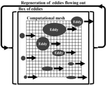
In this study, the SEM first proposed by Jarrin et al. (original SEM hereafter) [25,26] is used. In this method, a turbulent velocity field is obtained by the convection of eddies in a box set in advance and the superposition of fluctuations created by convecting eddies as shown in Fig. 1. The initial positions of eddies are determined using uniform random numbers so that distributions of them are not biased in the box. The turbulent velocity components ui obtained by the original SEM are expressed by the following equations.
(
)
1 1 ij N n n i ij j n u A f N = =
x−x (1)In the original SEM, the correlations between velocities in different directions are given using the Cholesky decomposition Aij of Reynolds stress tensor rij.
(
)
11 2 21 11 22 21 2 2 31 11 32 21 31 22 33 31 32 0 0 0 ij r A r A r A r A r A A A r A A = − − − − (2) εjnis a value that determines the positive or negative sign of the convecting eddy and it is given by a random number that follows the normal distribution with an average of 0 and a variance of 1. fσ
ij is a shape function,
which determines the shape of the fluctuation created by the convecting eddy.
3 3 1 1 2 2 1 1 2 2 3 3 1 1 1 ij n n n B i i i i i i x x x x x x f V
f
f
f
− − − = (3)The function f is the same for all eddies, and in this study the following Gaussian function is used.
( )
(
)
(
)
2 9 2 1 0 1 X Ce X f X X − = (4)( )
21
f
X dX
+ −=
(5)In addition, the size of the box where eddies are advected is determined by using the turbulent length scales.
( )
(
)
( )
(
)
,min , 1,2,3 ,max , 1,2,3 min max j j ij S i j S i j ij x x x x = − = + x x x x (6)All eddies are advected with a constant velocity Uc within the box. The position of eddy center at time t + dt is
(
)
( )
n n
c
t dt
+
=
t
+
dt
x
x
U
(7)The eddy flowing out of the box is regenerated at the inlet of the box, and its sign is also renewed.
Fig. 1 Schematic of the synthetic eddy method.
B. Divergence Free SEM
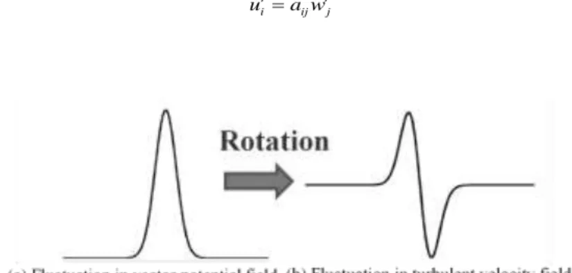
In addition to the original SEM described in the previous section, the DFSEM proposed by Sescu et al. [28] is adopted as a reconstruction method of a turbulent jet flow in this study. The DFSEM was developed with the aim of applying to the more accurate inflow boundary conditions for the computational aeroacoustics (CAA). Because it is based on the original SEM, the setting of the box where eddies advect and the regeneration of eddies outside the box are the same as those described in the previous section. The difference from the original SEM is that in the original SEM a turbulent velocity field is obtained directly from the superposition of
fluctuations produced by eddies, whereas in the DFSEM a vector potential field is generated from the superposition of them. Then, by taking the rotation of a vector potential field, a turbulent velocity field is obtained (see Fig. 2). Through such a process of the DFSEM, a fluctuation produced by one eddy necessarily has both positive and negative signs, therefore, fluctuations which satisfy the continuous equation are generated. The DFSEM is also suitable for modeling a quadrupole source generated by unsteady fluid motion like the jet noise. The turbulent velocity field generated by the DFSEM is expressed by the following equations.
(
x x x
1, ,
2 3)
(
x x x
1, ,
2 3)
=
v
Ψ
(8)(
)
1 1 2 2 3 3 1 2 3 1 , , , , n n n N n B n b b b x x V x x x x x x x N = L L L − − − =
Ψ ψ (9) 1 2 3 n=n +n +n ψ i j k (10)The shape of the fluctuation to be generated is determined by the following Gaussian function for all eddies. ( )2 3n r n n i C ie − = (11) 2 2 2 3 3 1 1 2 2 n n n n b b b x x x x x x r L L L − − − = + + (12)
(
)
21
ndxdydz
+ + + − − −
=
ψ
(13) εindetermines the positive or negative sign of the convecting eddy and is given by a random number that follows the normal distribution with an average of 0 and a variance of 1. In the DFSEM, the correlations between velocities in different directions are given by using Smirnov's method [34]. Smirnov's approach consists of the following steps.
1) The principal axis transformation is performed using eigenvectors of Reynolds stress tensor.
2) A turbulent velocity field v' satisfying the continuous equation is generated by the DFSEM in the principal coordinate system.
3) The eigenvalues ci of Reynolds stress tensor are used to impart the turbulence intensity.
i i i
w=c v (14)
4) Coordinate transformation is performed again to the original coordinate system, and a new turbulent velocity field u' is obtained.
i ij j
u=a w (15)
Fig. 2 Generation of turbulent velocity fluctuation in the DFSEM.
III. Reconstruction of Jet Turbulent Flow Field using SEM
A. Steady RANS Simulation of Turbulent Jet
The analysis of a high-subsonic turbulent round jet is performed by Reynolds-averaged Navier-Stokes equations solver implemented on the framework of BCM. The governing equations are discretized using the cell-centered finite volume method. The inviscid flux is computed by the simple low-dissipative advection upstream splitting (SLAU) [35] scheme. The third-order monotone upstream-centered schemes for conservation laws (MUSCL) [36] are employed to achieve high-order accuracy while satisfying the total variation diminishing condition. For time integration, the lower-upper symmetric Gauss–Seidel (LU-SGS) implicit method is employed [37]. The Chien’s k-ε turbulence model is used for a turbulence closure.
The targeted flow conditions are shown in Table 1. Mach number Mjet in the jet exit is 0.9 and Reynolds number Re with the sound speed a as a representative velocity is 4.44×10⁵. For ambient conditions, the freestream Mach number M∞ is set to 0.01 to stabilize the computation. Also, the following equations are applied as the jet inflow boundary condition.
jet 2 0.5 1 tanh 8 2 in D r D U U D r = − − (16) 0 in in V =W = (17) 2 2 r= y +z (18)
Here, the momentum thickness δθ is set to 0.1140×10⁻³ m at the jet inflow section [38]. For the inflow conditions of the turbulent kinetic energy kin and its dissipation rate εin, the following equations are used along the entire
inflow boundary [39] , where those values are varied based on the inlet velocity profile in Eq. (16). 2 2 1.5 in in k = I u (19)
(
2)
(
)
1, 000 in C k in I = (20) 0.01, 0.09 I = C = (21)Table 1 Flow conditions Jet exit conditions (Round jet)
Mach number Mjet = Ujet/a = 0.9
Reynolds number Re = ρaD/μ = 4.44×10⁵
Nozzle diameter D = 5.08×10⁻² m
Pressure p = 1013 hPa
Temperature T = 300 K
Ambient conditions Freestream Mach number M∞ = 0.01
Pressure p∞ = 1013 hPa
Temperature T∞ = 300 K
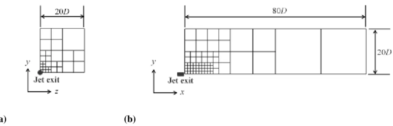
Figure 3 shows a computational domain and cube boundaries for the steady RANS simulation. The total number of cubes is 228, the total number of cells is 7,471,104, and the minimum cell size is 3.91×10⁻²D. Since
the axisymmetric computation whose center is the jet axis (y/D = 0, z/D = 0) is performed, the computational domain is one quarter of the size of the original flow field as shown in Fig. 3.
(a) (b)
Figure 4 shows the distributions of axial mean velocity U1 and turbulent kinetic energy k in the plane of z/D = 0. The potential core which is a constant velocity region is formed from the nozzle exit to a certain distance in the axial direction as in Fig. 4(a). Also, Fig. 4(b) shows that the shear layer is formed around the potential core, and large disturbance regions exist in the shear layer.
(a) (b)
Fig. 4 Computational results of steady RANS simulation, (a) axial mean velocity, (b) turbulent kinetic energy.
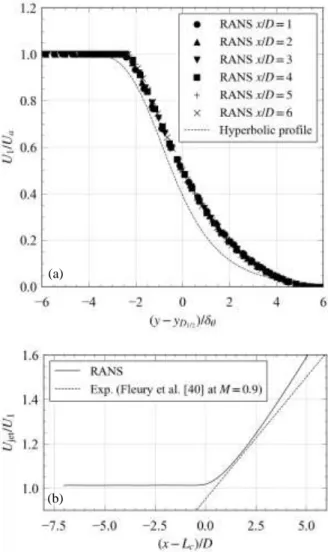
Next, Fig. 5 shows the detailed comparison of the axial mean velocity U1. In Fig. 5(a), the position y in the radial direction shown on the horizontal axis is non-dimensionalized using the half velocity diameter D1/2 and momentum thickness δθ, and computational results at various positions in the axial direction are summarized in
one figure. The classical velocity profile of jet represented by the following equation is also shown in this figure.
1 0.5 1 tanh 2 8 2 a U D y D U D y = − − (22)
In the computational result, the velocity distributions show the same shape at any positions in the axial direction. The computational result is generally in good agreement with the classical velocity profile. In Fig. 5(b), the experimental result by Fleury et al. [40] is used for computation. The potential core length Lc used in the
horizontal axis is set to 7 for both computational and experimental results. From this figure, a sudden increase of Ujet/U1 is observed at x > Lc, and its trend is consistent with the experimental result.
Furthermore, Fig. 6 shows the comparison of the turbulent kinetic energy k. The experimental results of Zaman et al. [39] are compared with the present simulation. As shown in Fig. 6, the computational results are in
50D 25D Jet exit 0.9 0.0 U1/a 50D 25D Jet exit 0.021 0.000 k/a2
good agreement with the experimental results. In the above validations, the results of the steady RANS simulation show good agreement with the experimental results. Therefore, the time-averaged components of the turbulent jet obtained in this section are reasonable as the input values to the SEM and the LEEs.
Fig. 5 Comparison of axial mean velocity U1, (a) profiles along the radial direction, (b) velocity decay
along the jet axis.
(a)
Fig. 6 Comparison of turbulent kinetic energy k, profiles along (a) the radial direction and (b) the jet axis.
B. Evaluation of Spatiotemporal Correlations of Generated Stochastic Turbulence
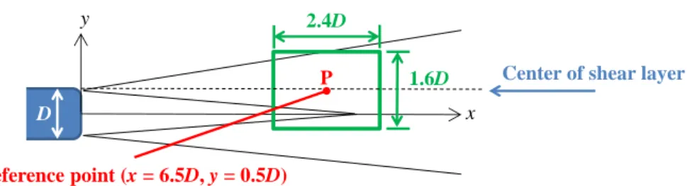
In this section, the SEM is applied to a part of turbulence developed within the shear layer. As shown in Fig. 7, a two-dimensional Cartesian mesh is considered on the plane of z/D = 0 (the green frame) for evaluating the spatiotemporal correlations. Then, a box for convecting eddies is set so as to surround it. Note that this two-dimensional mesh is different from the BCM mesh used in the steady RANS simulation, and it is a regular equidistant Cartesian mesh. The size of the evaluation domain is 2.4D in the axial direction (x direction) and
(a)
1.6D in the radial direction (y direction) with reference to the nozzle diameter D. Also, in order to investigate the space-time scales using the two-point two-time velocity correlation functions for the generated velocity fluctuations in Eq. (23), the reference point P is set at the center of the shear layer (x/D = 6.5, y/D = 0.5), and the computational domain is expanding centering on this point. Note that RANS simulation and the generation of turbulent fluctuations are conducted in the three-dimensional Cartesian mesh, that is, only the evaluation of turbulence statistics such as a two-point correlation is conducted on the two-dimensional plane along a jet centerline.
(
)
( ) (
)
( )
2(
)
2 , , , , , , i i ii i i u t u t R u t u t + + = + + x x ξ x ξ x x ξ (23)The number of grid points in the computational domain is 193 points in the x direction and 129 points in the y direction with Δx = Δy = 0.0125D. In both the original SEM and the DFSEM, input values from the background flow field are the same. Reynolds stress tensor rij and turbulent length scale Lb, are given by the following
equations. t 2 2 2 3 3 k ij i j ij ij ij k U r u u S k x
= = − − + (24) 1 2 j i ij j i U U S x x = + (25) 2 t k C = (26) 3 2 b b L k L f = (27)where the mean density ρ, mean velocity Ui, turbulent kinetic energy k, and its dissipation rate ε are input from
the results of the steady RANS simulation in the previous section. Cμ is the model constant of 0.09. fL
b in Eq.
(27) is a tuning parameter provided to adjust the turbulent length scale Lb, and in this section fL
b is set to 1.0.
From the experimental results by Fleury et al. [40], it has been confirmed that the entire turbulent structure in the shear layer advects along the center of the shear layer with a constant velocity of 0.6Ujet in the case of a subsonic jet. Therefore, the constant convection velocity Uc of the eddy center is given to all eddies by the
jet
0.6 , 0, 0
c c c
U = U V = W = (28)
For both the original SEM and the DFSEM, the number of eddies is 10,000, and the time step dt is set to 1.0 × 10⁻⁶ s.
Fig. 7 Computational domain for jet turbulent field reconstruction and a reference point of two-point two-time velocity correlation functions.
C. Spatial Correlations
Figure 8 shows the results when the time delay τ is zero, and large-scale turbulent structures in the shear layer depending on the flow field can be seen from this figure. For the validation of computational results, the experimental results by Fleury et al. at M = 0.9 [40] are used, where R11 levels are 0.8, 0.6, 0.4, 0.2, and 0.05 in black, and -0.05 and -0.1 in gray, and R22 levels are 0.8, 0.6, 0.4, 0.2, and 0.1 in black, and -0.1 and -0.2 in gray. First, the experimental result shows that the region with a relatively low positive correlation is greatly stretched in the direction inclined to a certain angle from the axial direction concerning the axial velocity correlation R11. This is because the turbulent structure in the shear layer is affected by the strong shear flow of the jet. Although this effect is not confirmed from the computational result of the original SEM, the inclination of the turbulent structure in the shear layer is consistent with the experimental result and the anisotropy of the jet is successfully reproduced in the DFSEM by generating the turbulent velocity field with coordinate transformation towards the principal axis direction of Reynolds stress tensor. However, the size of the entire turbulent structure is smaller than that of the experiment in both the original SEM and the DFSEM because of the lack of stretching of the region with low positive correlation. Therefore, the spatial scale of the generated turbulent field still has a difference from the actual flow. Second, concerning the radial velocity correlation R22, there are slightly negative
x y Reference point (x = 6.5D, y = 0.5D) 2.4D 1.6D D
Center of shear layer
regions on both sides of the region with high positive correlation in the experiment. This is one of the fundamental features of turbulence, and similar characteristic can be seen from the result of the DFSEM. Since the rotation of the vector potential field is taken to generate velocity fluctuations, one eddy always creates both positive and negative fluctuations in the DFSEM as shown in Fig. 2. For this reason, it is considered that the similar characteristics with the experiment appears in the result of the DFSEM.
Fig. 8 Isocontours of two-point velocity correlation functions R11 (τ = 0) in left and R22 in right, (a) the
experiment [40], (b) original SEM and (c) DFSEM. ξ1/D ξ2 /D ξ1/D ξ2 /D ξ1/D ξ2 /D
ξ
1/D
ξ
2/D
(a) Experiment [40] (b) Original SEM (c) DFSEMFigure 9 shows the distributions of turbulent kinetic energy (= 1 2⁄ u'̅̅̅̅̅̅) and Reynolds stress tensor riu'i ij
( =u'̅̅̅̅̅̅) obtained from the turbulent velocity field reconstructed by the SEM. The area shown in Fig. 9 iu'j corresponds to the domain enclosed by the green frame in Fig. 7. For the validation of computational results, input values from the RANS simulation are used. As shown in Fig. 9, the original SEM and the DFSEM successfully reproduce the values of the RANS. In the original SEM, r21 is well reproduced because velocities in different directions are correlated by the Cholesky decomposition of the Reynolds stress tensor. Therefore, it should be noted that it is not due to the reproduction of the inclination of the turbulent structures in the shear layer like the DFSEM.
(a)
(b)
(d)
Fig. 9 Distributions of turbulent kinetic energy k and Reynolds stress tensor rij (left: RANS, middle:
original SEM, right: DFSEM), (a) k, (b) r11, (c) r22 and (d) r21.
D. Time Correlations
In this section, the time delay τ is considered when calculating the velocity correlation functions Rii from the
generated turbulent field, and it is observed how the turbulent structures in the shear layer changes in time. Figure 10 shows the isocontours of the axial velocity correlation R11, where the contour levels are 0.8, 0.6, 0.4, 0.2, and 0.05 in black, and -0.05 and -0.1 in gray for the experiment of Fleury et al [40]. The entire turbulent structure in the shear layer convects to the downstream side with a constant velocity while almost maintaining its shape, size, and inclination in the experiment. In addition, the dissipation of the correlation coefficient occurs during convection at the central part of the turbulent structure. In the results of the original SEM and the DFSEM, the entire turbulent structure is convected with the same velocity as the experimental results while maintaining its shape and size. Nevertheless, the dissipation of the correlation coefficient is not reproduced. Therefore, it is necessary to separately give the dissipation effect of the turbulent structure in the shear layer to the generated velocity fluctuations by the SEM and adjust the time scale to the actual flow.
Fig. 10 Two-point two-time correlation function R11 (left: experiment [40], middle: original SEM, right:
DFSEM), (a) τUjet/D = 0, (b) τUjet/D = 0.4, (c) τUjet/D = 1.2, and (d) τUjet/D = 1.95.
E. SEM with decorrelation process
From the results of the time correlation in the previous section, it became clear that the turbulent velocity field generated by SEM does not include the dissipation effect of turbulent structures in the shear layer. In this section, a new method for reproducing the dissipation effect of the generated turbulent velocity fluctuations is
ξ1/D ξ2 /D ξ1/D ξ2 /D ξ1/D ξ2 /D ξ1/D ξ2 /D ξ1/D ξ2 /D ξ1/D ξ2 /D ξ1/D ξ2 /D ξ1/D ξ2 /D
ξ
1/D
ξ
2/D
(a) τUjet/D = 0
(b) τUjet/D = 0.4
(c) τUjet/D = 1.2
considered and its effect is investigated. In the original SEM and the DFSEM, the time dependency of generated velocity fluctuations is given only by a convection velocity Uc of the eddy center. On the other hand, the sign
(intensity) εjn of the eddy does not change during its advection through the box. Therefore, the increase of the decorrelation directly by dissipating the eddy intensity is attempted. The eddy intensity εin is directly dissipated in time using the following equations.
( )0,1
( )
(
)
n n it
i it dt
iG
i
=
−
+
(29) 2 , 1 i dt i e i i = − = − (30) i n i n k f = (31)As shown in the second term of Eq. (29), the random components are given by random numbers that follow a normal distribution with average of 0 and variance of 1. And fτi in Eq. (31) are tuning parameters, which are set
to fτ1 = 0.25, fτ2 = fτ3 = 0.5. Combining this method with the DFSEM, the same procedure as the previous section
is carried out. The conventional SEM/DFSEM does not consider the change of eddy strength (sign) during advection; therefore, it cannot represent the dissipation effect of turbulence. In this study, the decorrelation process is newly introduced to model the dissipation effect. Since SEM/DFSEM was originally proposed for providing an inlet boundary of LES, the dissipation of eddies during advection is not considered in the original SEM/DFSEM approaches.
Figure 11 shows the isocontours of the axial velocity correlation R11, where the contour levels are 0.8, 0.6, 0.4, 0.2, and 0.05 in black, and -0.05 and -0.1 in gray for the experiment of Fleury et al. [40]. In the results of combining the DFSEM and the decorrelation process, the dissipation of the correlation coefficient occurs at almost the same level as the experiment. In order to evaluate the applied effect more quantitatively, the Lagrangian decorrelation functions are calculated. They are shown in Fig. 12. In the calculation of the Lagrangian decorrelation functions, the correlation coefficients are obtained from two points, the reference point P and the point convecting to the downstream side with a constant velocity of 0.6 Ujet from the point P. For comparison, the experimental results by Fleury et al. [40] and the results of LES with same conditions performed in JAXA [4] are used. In both R11 and R22, the tendency of dissipation in present method is in good agreement with the experimental and LES results. Furthermore, Fig. 13 shows the distributions of turbulent kinetic energy
k obtained from the generated turbulent field. From this figure, it is shown that turbulent velocity fluctuations is
generated without destroying the original energy distributions even if the DFSEM is combined with the decorrelation process.
Fig. 11 Two-point two-time axial velocity correlation function R11 (left: the experiment [40], middle:
DFSEM, right: DFSEM with decorrelation process), (a) τUjet/D = 0, (b) τUjet/D = 0.4, (c) τUjet/D = 1.2,
and (d) τUjet/D = 1.95.
ξ1/D ξ2 /D ξ1/D ξ2 /D ξ1/D ξ2 /D ξ1/D ξ2 /D ξ1/D ξ2 /D ξ1/D ξ2 /D ξ1/D ξ2 /D ξ1/D ξ2 /D
ξ
1/D
ξ
2/D
(a) τUjet/D = 0
(b) τUjet/D = 0.4
(c) τUjet/D = 1.2
Fig.12 Lagrangian decorrelation functions Rii (x, ξ=0.6Ujetτ, τ) at reference point x/D = 6.5, y/D = 0.5,
(a) axial velocity correlation R11 and (b) radial velocity correlation R22.
(a) (b)
Fig. 13 Distributions of turbulent kinetic energy k, (a) RANS and (b) DFSEM with decorrelation process.
IV.
Jet-Noise Propagation Analysis Using SEM-LEE
A. Computational Setup
In this section, the jet-noise prediction using LEEs is carried out based on the validation results of the SEM in Section III. For the jet noise propagation analysis using LEEs, BCM-LEE solver developed by Fukushima [41-44] is used. The BCM-LEE solver has been validated by several test cases. The governing equations are the following linearized three-dimensional compressible Euler equations.
0 0 j j j j t x x − = − + Q Q Q A A S (32) 1 0 2 3 1 2 3 , p p U u U u U u
= = Q Q (33) 1 2 3 1 2 3 1 1 2 2 2 2 0 3 3 2 1 2 3 1 2 3 0 0 0 0 0 0 0 0 0 0 0 0 0 0 , 0 0 0 0 0 0 0 0 j j j j j j j j j j j j j j j j j j j j j j j j j j j j j j u u p U U U u u p p U U u p p p − − = = − A A (34)In this study, the following equations based on the Lighthill tensor [45]are used for the source term S in Eq. (32). 1 1 2 2 3 3 0 0 S S S S S S − = − − S (35) 0 0 , i j i j i i j j u u u u S S x x = − = − (36)
The turbulent velocity field fluctuations by SEM are directly input to these equations.
The governing equations are discretized by the fourth-order dispersion relation preserving scheme in space and the six-stage fourth-order Runge-Kutta scheme in time. The buffer zone boundary condition is employed for outer boundaries to suppress reflecting noise. A solid wall of the jet exit is handled by the immersed boundary method. As mentioned earlier, we use multi-level Cartesian mesh called BCM to cover the computational domain.
Figure 14 shows the computational domains and cube boundaries for LEE computation. As shown in Fig. 14, the computational domain is [-15D, 65D] in the x direction, [-20D, -20D] in the y direction, and [-10D, 10D] in the z direction. The nozzle exit center is the origin in this domain. The total number of cubes is 1,296, the total
number of cells is 42,467,328, and the minimum cell size is 3.9×10⁻²D. The inner buffer zone boundaries are set
at the boundaries of region divided by the minimum cell, and they are x/D = [-2.5, 22.5], y/D = [-2.5, 22.5], and
z/D = [-2.5, 2.5]. By increasing the cube size between the inner buffer zone boundaries and the outer boundaries,
the artificial damping of sound waves works more efficiently. The measurement points of pressure are set at x/D = 0, 5, 10, 15 along the line of y/D = 7.5 and z/D = 0, and the pressure fluctuations are obtained directly from the results of this LEE computation. The region generating the turbulent velocity fluctuations using the SEM is
x/D = [0, 12], y/D = [-1.5, 1.5], and z/D = [-1.5, 1.5], and it is sufficiently large to cover the entire shear layer
which is the main noise source. The size and strength of eddies are recalculated based on the advected position, local flow variables including turbulent kinetic energy and dissipation rate from the RANS flow field for each time step. The number of eddies is 50,000 and the values of Reynolds stress tensor, turbulent length scale, and the convection velocity of the eddy center, which are input parameters to the SEM, are given in the same way as in Section III. We varied the number of eddies and confirmed that the larger number of eddies improves turbulent statistics and the predicted noise by LEE. On the other hand, it is also true that the large number of eddies increases the overall computational cost; therefore, we set the number to 50,000 to keep the benefit of SEM/DFSEM turbulence generation.
(a) (b) 20D z y Jet exit 80D 40D x y Jet nozzle
Pressure measurement points (y/D = 7.5, z/D = 0) Inner buffer zone boundaries
Fig. 14 Computational domains and cube boundaries for LEE computation, views from (a) -x direction and (b) +z direction.
In this section, the computations of the six cases shown in Table 2 are carried out. In case 5, the shear effect due to the mean flow and the dissipation effect of the turbulent structures are given to the turbulent velocity field using the DFSEM with the decorrelation process. Furthermore, the dissipation effect of the turbulent structures in the shear layer is adjusted to the actual flow by setting the tuning parameters in Eq. (31) to fτ1 = 0.25 and fτ2 =
fτ3 = 0.5 as in the validation in Section III.
Table 2 Computational conditions for LEE computation
Case Sound source reconstruction
Reynolds stress anisotropic tensor (Shear effect due to
mean flow)
Dissipation effect of turbulent structures
Original SEM None None
2 Original SEM Exist None
3 DFSEM None None
4 DFSEM Exist None
5 DFSEM with decorrelation
process Exist
Exist
(fτ1 = 0.25, fτ2 = 0.5, fτ3 = 0.5) 6 DFSEM with decorrelation
process Exist
Exist
(fτ1 = 125, fτ2 = fτ3 = 250)
B. Original SEM and DFSEM
In this section, the results of using the original SEM (cases 1 and 2) and the DFSEM (cases 3 and 4) are explained, where cases 2 and 4 consider the anisotropic components of Reynolds stress tensor when generating velocity fluctuations. The velocity correlations in different directions are taken into account and the shear effect due to the mean flow is given by the anisotropic components. However, r21 and r31 which represent the shear effect are provided by correlating between velocities in different directions using the Cholesky decomposition of the Reynolds stress tensor in the original SEM. Therefore, it should be noted that they are not due to the reproduction of the inclination of the turbulent structure in the shear layer like the DFSEM.
Figure 15 shows the distributions of instantaneous pressure fluctuations on the plane of z/D = 0. It is observed that very strong noise is generated from the nozzle exit and propagate toward outer boundaries in cases 1 and 2. Apart from this, very large fluctuations that are different from acoustic waves are developed along the jet axis. Second, the noise generated from the nozzle exit are reduced in cases 3 and 4, although large fluctuations that develop along the jet axis are also confirmed. The shear effect of the turbulent velocity field in the sound source is not confirmed only by these figures. The strong noise might come from the strong disturbance locally appeared in the jet core due to insufficient number of eddies. The eddies distributed in the jet core should not work as noise source by canceling each other; however, they sometimes exhibit strong disturbance because the superposition of eddies is weakened due to the insufficient number of eddies in the case of SEM. It is improved in the DFSEM as in Fig. 15(c) and (d).
(a) (b)
(c) (d)
Fig. 15 Distributions of instantaneous pressure fluctuations in the plane of z/D = 0 for (a) case 1, (b) case 2, (c) case 3, and (d) case 4.
The sound pressure spectrums obtained from the measured pressure fluctuations are shown in Fig. 16. Since there is no significant difference in the spectral shape between cases 1, 3 and cases 2, 4, it is clear that the shear
25D 12.5D Jet exit 0.001 -0.001 p 25D 12.5D Jet exit 0.001 -0.001 p 25D 12.5D Jet exit 0.001 -0.001 p 25D 12.5D Jet exit 0.001 -0.001 p
frequency becomes higher at any measurement points in the experiment of Bogey et al. [46]. However, the high frequency components around the Strouhal number St ≈ 6.4 greatly exceed the experimental results in cases 1 and 2, and the spectral shape is obviously different. This is due to the very strong noises generated from the nozzle exit seen in Fig. 15. There is a possibility that the accuracy of the generated velocity fluctuations is not sufficient due to the shortage of the number of eddies near the nozzle exit. It is also considered that the dissipation effect of the turbulent structures is not sufficient. On the other hand, the noise level on the high frequency side of St > 0.8 decreases by about 30dB in cases 3 and 4 compared to the results of cases 1 and 2 due to the absence of the strong noise from the nozzle exit.
Fig. 16 Sound pressure spectrums of cases 1 to 4, (a) x/D = 0, (b) x/D = 5, (c) x/D = 10, and (d) x/D = 15.
Figure 17 shows the distributions of instantaneous source term component S1 - S̅ of LEEs on the plane of 1
z/D = 0. Figures 17(a) and (b) correspond to cases 1 and 3, respectively. The values of the sound source term in
(a) (b)
case 3 are smaller than the in case 1 in the main sound source part in the shear layer. Since the magnitude of the velocity fluctuations input to Eq. (35) is determined so that the turbulent energy distributions can be reconstructed accurately in both cases, this difference is caused by whether the velocity fluctuations are made to satisfy the continuity equation or not. When the velocity fluctuations are generated so as to satisfy the continuity equation, the intensity of the sound source becomes weaker than the case where the continuity equation is not satisfied. As a result, a reduction of the noise level in particular in the high frequency components occurs. The eddies are also distributed in the jet core as in Fig. 17(a), which may be beneficial for applying the present approach to more complex configurations because there is no need to exactly define an eddy box depending on a background flow field. The eddies are basically negligible because the strength of each eddy, which is calculated by local k and , is small in the core area; however, they could cause the strong disturbance, as mentioned in the response to comment 5, due to the breakage of cancelation of eddies. Such defect does not appear in DFSEM because the turbulent velocity field is not directly obtained from superimposed eddies, instead we take a rotation of the vector potential as in Eq. (10).
(a) (b)
Fig. 17 Distributions of instantaneous source term components on the plane of z/D = 0 for (a) case 1 and (b) case 3.
C. DFSEM with decorrelation process
In this section, the results of cases 5 and 6 in which the dissipation effect of the turbulent structures in the shear layer is given to the turbulent velocity fluctuations are explained. In case 5, the dissipation effect of the turbulent structures is adjusted to the actual flow by setting the tuning parameters in Eq. (31) to fτ1 = 0.25 and fτ2
= fτ3 = 0.5. In case 6, the time delay is increased by setting the tuning parameters to fτ1 = 125 and fτ2 = fτ3 = 250.
12.5D 3D Jet exit 0.5 -0.5 1 1 S−S 12.5D 3D Jet exit 0.5 -0.5 1 1 S−S
Figure 18 shows the distributions of instantaneous pressure fluctuations and source term components in case 5. As shown in Fig. 18(a), the distribution of instantaneous pressure fluctuations is quite different from the results of cases 3 and 4 only using the DFSEM, and very strong sound waves are radiated from the inside of the shear layer. The sound source term in Fig. 18(b) is similar to that of case 3 in Fig. 17(b). The computational results of case 6 are shown in Fig. 19. As shown in Fig. 19(a), the strong sound radiation from the inside of the shear layer is reduced by setting the dissipation time to be longer than case 5. Here, the distribution of the sound source term in Fig. 19(b) is similar to that of cases 3 and 5. Thus, very strong sound waves are radiated due to the dissipation effect of the turbulent structures in case 5.
a) b)
Fig. 18 Results of case 5 on the plane of z/D = 0, the distribution of (a) instantaneous pressure fluctuations and (b) instantaneous source term components.
a) b)
Fig. 19 Results of case 6 on the plane of z/D = 0, the distribution of (a) instantaneous pressure fluctuations and (b) instantaneous source term components.
25D 12.5D Jet exit 0.001 -0.001 p 12.5D 3D Jet exit 0.5 -0.5 1 1 S−S 25D 12.5D Jet exit 0.001 -0.001 p 12.5D 3D Jet exit 0.5 -0.5 1 1 S−S
Figure 20 shows the sound pressure spectrums. In case 5, the final estimated noise levels exceed the experimental results by 20dB to 30dB at all measurement points considered here, although the turbulent statistics are brought closest to the experiment. Similar results have been reported in the computation using the SNGR model of Lafitte et al. [12]. In case 6, where the time taken to dissipate the turbulent structures is longer than case 5, the noise levels are reduced at all of measurement points, and the spectral shapes also become consistent with the experiment. Although it is possible to reduce the noise values by adjusting the tuning parameter fτ
i as in
case 6, the parameter values are 500 times larger than case 5. Therefore, the time until the dissipation of the turbulent structures also takes about 500 times longer than case 5 from Eqs. (29), (30) and (31). In other words, the time scale of case 6 is very different from the experiment. The tuning parameter controls the dissipation effect of eddies, i.e., the larger parameter values decreases the dissipation effect. In this study, the dissipation effect is realized by adding a random component to the strength of eddy, which could be a reason why the turning parameter needs to be such large. There would be alternative ways to introduce the dissipation effect of eddies without having such large values of the tuning parameters.
Fig. 20 Sound pressure spectrums of cases 5 and 6 at (a) x/D = 0, (b) x/D = 5, (c) x/D = 10, and (d) x/D = 15.
V. Conclusions
The efficient jet-noise prediction tool using the SEM was developed and the influence of the reproduced turbulent statistics on the noise estimation accuracy was investigated in the present study. First, the accuracy of the reconstructed flow field by the SEM was validated using various turbulence statistics. With the DFSEM, the inclination of two-point velocity correlations which shows the strong shear effect due to the background shear flow was reproduced. Furthermore, the dissipation effect of the turbulence was taken into account by combining the DFSEM with a procedure to increase the time-decorrelation of the generated velocity fluctuations. In the DFSEM with the decorrelation process, the intensity of the turbulence is also accurately reconstructed without the loss of the local turbulent kinetic energy. Second, the influence of turbulence statistics on far-field jet-noise
(a) (b)
was investigated by LEEs, where the velocity fluctuations generated by the SEM were used in the sound source term of LEEs. The estimated noise appeared much larger than the experimental value when parameters of the SEM were set based on the experiment. On the other hand, the sound pressure spectra agreed well with the experiment by increasing the time scale. With the present stochastic noise prediction framework based on the SEM, turbulence statistics and far-field sound pressure spectra are correlated, which would help to modify parameters in stochastic noise generation to achieve desired far-field sound pressure spectra. We expect that once turning parameters are defined based on reference simulation or experiment, the fast-time noise prediction can be conducted only using a RANS flow field. It is of course necessary to explore how valid the predicted noise is in the different flow configuration from the reference condition. Further validation would be of our future work before applying this approach to more complex flow configurations.
Acknowledgments
We thank computational resources provided by the Institute of Fluid Science, Tohoku University.
References
[1] Dickson, N., “ICAO Noise Standards,” ICAO Symposium on Aviation and Climate Changes, 2013. [2] Depuru Mohan, N. K., and Dowling, A. P., “Jet-Noise-Prediction Model for Chevrons and Microjets,” AIAA
Journal, Vol. 54, No. 12, pp. 3928-3940, 2016, DOI: 10.2514/1.J054546.
[3] Zaman, K. B. M., “Jet Noise Reduction by Microjets – A Parametric Study,” AIAA Paper 2009-3129, 2009. DOI: 10.2514/6.2009-3129.
[4] Ikeda, T., Yamamoto, K., and Amemiya K., “The Frequency-Domain Formulations of the Quadrupole Correction for the Ffowcs Williams Hawkings Integration,” AIAA Paper 2016-2794, 2016, DOI: 10.2514/6.2016-2794.
[5] Kraichnan, R., “Diffusion by a Random Velocity Field,” Physics of Fluids, Vol. 13, No. 1, pp. 22–31, 1970, DOI: 10.1063/1.1692799.
[6] Karweit, M., Blanc-Benon, P., Juvé, D., and Comte-Bellot, G., “Simulation of the Propagation of an Acoustic Wave Through a Turbulent Velocity Field: A Study of Phase Variance,” Journal of the Acoustical
[7] Bechara,W., Bailly, C., Lafon, P., and Candel, S., “Stochastic Approach to Noise Modeling for Free Turbulent Flows,” AIAA Journal, Vol. 32, No. 3, pp. 455–463, 1994, DOI: 10.2514/3.12008.
[8] Bailly, C., and Juvé, D., “A Stochastic Approach to Compute Subsonic Noise Using Linearized Euler’s Equations,” 5th AIAA/CEAS Aeroacoustics Conference, AIAA Paper 1999-1872, May 1999, DOI: 10.2514/6.1999-1872.
[9] Ewert, R., “Broadband Slat Noise Prediction Based on CAA and Stochastic Sound Sources from a Fast Random Particle Mesh (RPM) Method,” Computers and Fluids, Vol. 37, No. 4, pp. 369–387, 2008, DOI: 10.1016/j.compfluid.2007.02.003.
[10] Billson, M., Eriksson, L., and Davidson, L., “Jet Noise Prediction Using Stochastic Turbulence Modeling,” 9th AIAA/CEAS Aeroacoustics Conference, AIAA Paper 2003-3282, May 2003, DOI: 10.2514/6.2003-3282.
[11] Lafitte, A., Laurendeau, E., La Garrec, T., and Bailly, C., “A Study Based on the Sweeping Hypothesis to Generate Stochastic Turbulence,” 17th AIAA/CEAS Aeroacoustics Conference, AIAA Paper 2011-2888, June 2011, DOI: 10.2514/6.2011-2888.
[12] Lafitte, A., Laurendeau, E., Le Garrec, T., and Bailly, C., “Prediction of Subsonic Jet Noise Relying on a Sweeping Based Turbulence Generation Process,” 18th AIAA/CEAS Aeroacoustics Conference, AIAA Paper 2012-2149, June 2012, DOI: 10.2514/6.2012-2149.
[13] Lafitte, A., Garrec, T., Bailly, C., and Laurendeau, E., “Turbulence Generation from a Sweeping-Based Stochastic Model,” AIAA Journal, Vol. 52, No. 2, February 2014, DOI: 10.2514/1.J052368.
[14] Careta, A., Sagués, F., and Sancho, J., “Stochastic Generation of Homogenous Isotropic Turbulence with Well-Defined Spectra,” Physical Review E, Vol. 48, No. 3, pp. 2279–2287, 1993, DOI: 10.1103/PhysRevE.48.2279.
[15] Ewert, R., and Edmunds, R., “CAA Slat Noise Studies Applying Stochastic sound Sources Based on Solenoidal Filters,” 11th AIAA/CEAS Aeroacoustics Conference, AIAA Paper 2005-2862, May 2005, DOI: 10.2514/6.2005-2862.
[16] Ewert, R., Dierke, J., Siebert, J., Neifeld, A., Appel, C., Siefert, M., and Kornow, O., “CAA Broadband Noise Prediction for Aeroacoustic Design,” Journal of Sound and Vibration, Vol. 330, No. 17, pp. 4139– 4160 , 2011, DOI: 10.1016/j.jsv.2011.04.014.
[17] Dieste, M., and Gabard, G., “Broadband Fan Interaction Noise Using Synthetic Inhomogeneous Non-Stationary Turbulence,” 17th AIAA/CEAS Aeroacoustics Conference, AIAA Paper 2011-2708, June 2011, DOI: 10.2514/6.2011-2708.
[18] Dieste, M., and Gabard, G., “Random Particle Methods Applied to Broadband Fan Interaction Noise,” Journal of Computational Physics, Vol. 231, No. 24, pp. 8133–8151, 2012, DOI: 10.1016/j.jcp.2012.07.044. [19] Dieste, M., and Gabard, G., “Synthetic Turbulence Applied to Broadband Interaction Noise,” 15th
AIAA/CEAS Aeroacoustics Conference, AIAA Paper 2009-3267, May 2009, DOI: 10.2514/6.2009-3267. [20] Dieste, M., and Gabard, G., “Random-Vortex-Particle Methods for Broadband Fan Interaction Noise,” 16th AIAA/CEAS Aeroacoustics Conference, AIAA Paper 2010-3885, June 2010, DOI: 10.2514/6.2010-3885. [21] Ewert, R., Dierke, J., Pott-Pollenske, M., Appel, C., Edmunds, R., and Sutcliffe, M., “CAA-RPM Prediction and Validation of Slat Setting Influence on Broadband High-Lift Noise Generation,” 16th AIAA/CEAS Aeroacoustics Conference, AIAA Paper 2010-3883, June 2010, DOI: 10.2514/6.2010-3833.
[22] Siefert, M., and Ewert, R., “Sweeping Sound Generation in Jets Realized with a Random Particle-Mesh Method,” 15th AIAA/CEAS Aeroacoustics Conference, AIAA Paper 2009-3369, May 2009, DOI: 10.2514/6.2009-3369.
[23] Neifeld, A., and Ewert, R., “Jet Mixing Noise from Single Stream Jets Using Stochastic Source Modeling,” 17th AIAA/CEAS Aeroacoustics Conference, AIAA Paper 2011-2700, June 2011, DOI: 10.2514/6.2011-2700.
[24] Ewert, R., Neifeld, A., and Fritzsch, A., “A 3-D Modal Stochastic Jet Noise Source Model,” 17th AIAA/CEAS Aeroacoustics Conference, AIAA Paper 2011-2887, June 2011, DOI: 10.2514/6.2011-2887. [25] Jarrin, N., Benhamadouche, S., Laurence, D., and Prosser, R., “A Synthetic-Eddy-Method for Generating Inflow Conditions for Large-Eddy Simulation,” International Journal of Heat and Fluid Flow, Vol. 27, No. 4, pp. 585–593, 2006, DOI: 10.1016/j.ijheatfluidflow.2006.02.006.
[26] Jarrin, N., Prosser, R., Uribe, J., Benhamadouche, S., and Laurence, D., “Reconstruction of Turbulent Fluctuations for Hybrid RANS/LES Simulations Using a Synthetic-Eddy Method,” International Journal of Heat and Fluid Flow, Vol. 30, No. 3, pp. 435–442, 2009, DOI: 10.1016/j.ijheatfluidflow.2009.02.016. [27] Poletto, R., Craft, T., and Revell, A., “A New Divergence Free Synthetic Eddy Method for the Reproduction
of Inlet Flow Conditions for LES,” Flow, Turbulence and Combustion, Vol. 91, No. 3, pp. 519-539, 2013, DOI: 10.1007/s10494-013-9488-2.
[28] Sescu, A., and Hixon, R., “Generation of Divergence-Free Synthetic Turbulence Velocity Fields for LES/CAA Applications,” 50th AIAA Aerospace Sciences Meeting, AIAA Paper 2012-0466, 2012, DOI: 10.2514/6.2012-466.
[29] Fukushima, Y., “Efficient Jet Noise Prediction Using Synthetic Eddy Method and Block-Structured Cartesian Mesh,” 29th Congress of the International Council of the Aeronautical Sciences, 2014.
[30] Nakahashi, K., “Building-Cube Method for Flow Problems with Broadband Characteristic Length,” Computational Fluid Dynamics 2002, pp. 77-81, 2003, DOI:10.1007/978-3-642-59334-5_7.
[31] Nakahashi, K., and Kim, L., “High-Density Mesh Flow Computations by Building-Cube Method,” Computational Fluid Dynamics 2004, pp. 121-126, 2006, DOI: 10.1007/3-540-31801-1_13.
[32] Ishida, T., Takahashi S., and Nakahashi, K., “Efficient and Robust Cartesian Mesh Generation for Building-Cube Method,” Journal of Computational Science and Technology, Vol. 2, No. 4, pp. 435-446, 2008, DOI: 10.1299/jcst.2.435.
[33] Nishimoto, S., Sasaki, D., and Nakahashi, K., “RANS Simulation around Airfoils Using Building-Cube Method,” 48th AIAA Aerospace Sciences Meeting, AIAA Paper 2010-710, 2010, DOI: 10.2514/6.2010-710.
[34] Smirnov, A., Shi, S., and Celik, I., “Random Flow Generation Technique for Large Eddy Simulations and Particle-Dynamics Modeling,” Journal of Fluids Engineering, Vol. 123, No. 2, pp. 359-371, 2001, DOI: 10.1115/1.1369598.
[35] Shima, E., and Kitamura, K., “On New Simple Low-Dissipation Scheme of AUSM-Family for All Speeds,” 47th AIAA Aerospace Sciences Meeting, AIAA Paper 2009-136, 2009, DOI: 10.2514/6.2009-136.
[36] van Leer, B., “Towards the Ultimate Conservation Difference Scheme. IV. A New Approach to Numerical Convection,” Journal of Computational Physics, Vol. 23, No.3, pp. 276-299, 1977, DOI: 10.1016/0021-9991(77)90095-X.
[37] Yoon, S., and Jameson, A., “Lower-Upper Symmetric-Gauss Seidel Method for the Euler and Navier-Stokes Equations,” AIAA Journal, Vol. 26, No. 9, pp. 1025–1026, 1988, DOI: 10.2514/3.10007.
[38] Faghani, E., Maddahian, R., Faghani, P., and Farhanieh, B., “Numerical Investigation of Turbulent Free Jet Flows Issuing from Rectangular Nozzles: the Influence of small Aspect Ratio,” Archive of Applied Mechanics, Vol. 80, No. 7, pp. 727-745, 2010, DOI: 10.1007/s00419-009-0340-z.
[39] Zaman, K.M.B.Q., Wang, F.W., and Georgiadis, N.J., “Noise, Turbulence, and Thrust of Subsonic Freejets from Lobed Nozzles, AIAA Journal, Vol. 41, No. 3, pp. 398-407, 2003, DOI: 10.2514/2.1990.
[40] Fleury, V., Bailly, C., Jondeau, E., Michard, M., and Juvé, D., “Space–Time Correlations in Two Subsonic Jets Using Dual Particle Image Velocimetry Measurements,” AIAA Journal, Vol. 46, No. 10, pp. 2498– 2509, 2008, DOI: 10.2514/1.35561.
[41] Fukushima, Y., Daisuke, S., and Nakahashi, K., “Cartesian Mesh Linearized Euler Equations Solver for Aeroacoustic Problems around Full Aircraft,” International Journal of Aerospace Engineering, vol. 2015, Article ID 706915, 18 pages, 2015, DOI: 10.1155/2015/706915.
[42] Fukushima, Y., Misaka, T., Obayashi, S., Jeong, S., Sasaki, D., and Nakahashi, K., “CFD-CAA Coupled Computation of Fan Noise Propagation from Engine Nacelle Based on Cartesian Mesh Method,” 19th AIAA/CEAS Aeroacoustics Conference, AIAA Paper 2013-2020, 2013, DOI: 10.2514/6.2013-2020. [43] Fukushima, Y., Misaka, T., Obayashi, S., Sasaki, D., and Nakahashi, K., “The Numerical Analysis of
Forward Fan Noise Shielding Effect on the Over-the-Wing Nacelle Configuration,” 52nd Aerospace Sciences Meeting, AIAA Paper 2014-0720, 2014, DOI: 10.2514/6.2014-0720.
[44] Fukushima, Y., Misaka, T., Obayashi, S., Sasaki, D., Nakahashi, K., “Wavenumber Optimized Immersed Boundary Method for AeroAcoustic Analysis Based on Cartesian Mesh Method,” AIAA Journal, Vol. 54, No, 10, pp. 2988-3001, 2016, DOI: 10.2514/1.J053958.
[45] Bogey, C., Bailly, C., and Juve, D., “Computation of Flow Noise Using Source Terms in Linearized Euler’s Equations,” AIAA Journal, Vol. 40, No. 2, pp. 235-243, 2002, DOI: 10.2514/2.1665.
[46] Bogey, C., Barré, S., Fleury, V., Bailly, C., and Juvé, D., “Experimental Study of the Spectral Properties of Near-field and Far-field Jet Noise,” International Journal of Aeroacoustics, Vol. 6, No. 2, pp. 73-92, 2007, DOI: 10.1260/147547207781041868.


![Fig. 8 Isocontours of two-point velocity correlation functions R 11 (τ = 0) in left and R 22 in right, (a) the experiment [40], (b) original SEM and (c) DFSEM](https://thumb-ap.123doks.com/thumbv2/123deta/5921164.1051221/18.918.167.755.321.930/isocontours-point-velocity-correlation-functions-experiment-original-dfsem.webp)


