東北大学機関リポジトリTOUR

Recruitment and entrainment processes of woody

debris caused by disastrous landslides and

debris flows

著者

Thapthai Chaithong

学位授与機関

Tohoku University

学位授与番号

11301甲第18808号

Recruitment and Entrainment Processes of Woody Debris Caused

by Disastrous Landslides and Debris Flows

斜面崩壊による流木発生メカニズムの解明

Thapthai Chaithong

(ID NO. B6GD4001)

Department of Frontier Science for Advanced Environment

Graduate School of Environmental Studies

TOHOKU UNIVERSITY

JAPAN

2

ACKNOWLEDGEMENTS

Firstly, I would like to express my sincere appreciation to my thesis advisor, Associate Professor Daisuke Komori, for giving me the opportunity to be part of his research group at the Graduate School of Environmental Studies, Tohoku University, and continuously following my PhD thesis. His guidance helped me throughout the research and writing of this thesis. I would like to sincerely thank Professor So Kazama for his guidance and valuable suggestions for improving my research. I also thank Assistant Professor Yoshiya Touge for his helpful comments on my thesis. I am deeply indebted to Associate Professor Suttisak Soralump from Kasetsart University, Thailand, who introduced me to Associate Professor Daisuke Komori and supported me in developing the shallow landslide model. Without his invaluable assistance, it would not have been possible to complete this thesis. I am also immensely grateful to Associate Professor Apiniti Jotisankasa from Kasetsart University, Thailand, for helping me acquire an understanding of the behaviour of unsaturated soil.

In addition to my advisor, I would like to thank the rest of my thesis committee – Professor Yu-You Li, Professor Tomoki Nakaya and Associate Professor Isao Murata – for their insightful comments and encouragement to improve this dissertation. Furthermore, the valuable criticism, questions and comments of all faculty and colleagues at the Hydro-Environmental Systems Laboratory, Disaster Potential Laboratory, Environmental Hydrodynamics Laboratory, Tsunami Laboratory and Laboratory of Remote Sensing and Geoinformatics for Disaster Management during the doctoral seminar (D-semi) are appreciated. Particular thanks go to Professor Hitoshi Tanaka for his comments and challenging questions, which encouraged me to refine my research. Moreover, I would like to offer my special thanks to all the faculty and administrative staff as well as my colleagues at the Graduate School of Environmental Studies, Tohoku University, for their support throughout this study. I am indebted to the administrative staff at the Hydro-Environmental Systems Laboratory for their assistance in innumerable tasks. I also wish to thank the members of the Hydro-Environmental Systems Laboratory for their support throughout my study, especially Mr. Yuto Sukegawa and Mr. Yuta Sugawara. For the scholarship that allowed me to pursue my doctoral course, I would like to thank the Japanese Ministry of Education, Culture, Sports, Science and Technology (MEXT).

I would also like to extend my gratitude to the faculty and technicians of the Geotechnical Laboratory of the Department of Civil and Environmental Engineering, Tohoku University, for helping me to access the resources required to conduct the research for this thesis.

My profoundest appreciation goes to Ms. Tipawan Nipakakul for her love and support throughout this study. I also thank my instructors and friends at Buranarumluk School,

Sendai-3

Thai Student, Kasetsart University and King Mongkut’s University of Technology North Bangkok.

Finally, nobody has been more essential to me in the pursuit of this study than the members of my family. My deepest gratitude goes to my parents for their incomparable support and unconditional love.

4

Recruitment and entrainment processes of woody debris caused by disastrous landslides and debris flows

ABSTRACT: Woody debris is a natural component which plays both positive and negative roles in the ecosystem, such as providing habitats for vertebrates, insects and microorganisms in aquatic and forest ecosystems or increasing the destructive power of floods or debris flows. Understanding the volume and dynamics of woody debris can help predict the roles of, or prevent hazards from, woody debris. The major objectives of this study are to understand the process of woody debris recruitment and the mechanisms of woody debris entrainment related to landslides and debris flows. To achieve these aims, this study is divided into five main steps: (1) developing a rainfall-induced shallow landslide model for predicting areas of instability; (2) coupling the rainfall-induced shallow landslide model and forest properties to estimate the volume of woody debris caused by shallow landslides; (3) developing the sliding block model for debris flow runout based on Newton’s second law of motion and the concept of momentum to explain the entrainment of woody debris due to debris flows; (4) developing the tree stability model to evaluate the stability of trees related to the forces of debris flows; and (5) evaluating the woody debris deposition zone related to rainfall-induced landslides and debris flows using

the integrated rainfall-induced shallow landslide and GIS-based debris flow runout models.

The rainfall-induced shallow landslide model integrates the hydrologic and infinite slope stability models. To verify the performance of the rainfall-induced shallow landslide model, this study used two historical landslide cases in Thailand and Japan. The data show that the rainfall-induced shallow landslide model is able to predict landslides at the regional scale.

To estimate the woody debris recruitment caused by rainfall-induced shallow landslides, this study combined unstable areas as determined by the shallow landslide model with tree density data and observational data following the occurrence of a landslide. The study site is a sub-catchment of the Omoto River watershed in Iwaizumi, Iwate Prefecture, Japan, which was struck by Typhoon Lionrock in 2016. The results show that the proposed procedure can estimate the woody debris recruitment a watershed; however, the procedure underestimates the amount of woody debris recruited when compared to field-based measurements.

The mechanism of woody debris entrainment by debris flows is described using the momentum changes of debris flows due to the entrainment of woody material. In this study, such momentum changes are termed the momentum of entrainment. Moreover, debris flows can destroy trees in the flow path. The tree stability index is proposed to identify the stability of trees attacked by debris flows. The tree stability index is the ratio of the resisting shear force to the driving shear force. The results show that the tree stability index is effective at predicting

5

the stability of trees.

The area in which woody debris is deposited can be predicted using the coupled rainfall-induced shallow landslide and debris flow runout models. This study uses the debris flow runout model proposed by Hunt (1994), which treats debris flows as laminar and as a Newtonian fluid. The conditions of woody debris movement and deposition are based on the individual log motion concept proposed by Braudrick and Grant (2000), Haga et al. (2002) and Mazzorana et al. (2010). The case study for evaluating the performance of the proposed concept is a landslide and debris flow event that took place in the city of Kure, Hiroshima, Japan, in July 2018. According to the calculation, the integrated model is able to predict the deposition areas of woody debris as a result of debris flows.

6

Table of Contents

CHAPTER 2: RESEARCH METHODS AND DATA SOURCES ... 14

CHAPTER 3: A MODEL TO ASSESS RAINFALL-INDUCED SHALLOW LANDSLIDES ... 18

CHAPTER 4: ESTIMATING WOODY DEBRIS RECRUITMENT IN A STREAM CAUSED BY A TYPHOON-INDUCED LANDSLIDE: A CASE STUDY OF TYPHOON LIONROCK IN IWAIZUMI, IWATE PREFECTURE, JAPAN ... 32

CHAPTER 5: A MODEL FOR ASSESSMENT OF TREE STABILITY AND ENTRAINMENT OF WOODY DEBRIS BY FLOW SLIDES AND SHALLOW SLOPE FAILURE... 36

CHAPTER 6: SIMULATION OF WOODY DEBRIS DEPOSITION USING INTEGRATED RAINFALL-INDUCED SHALLOW LANDSLIDES MODEL AND DEBRSI FLOW RUNOUT MODEL ... 45

CHAPTER 7: CONCLUSIONS AND RECOMMENDATIONS ... 53

7

LIST OF ABBREVIATIONS

ALOS-PALSAR Advanced Land Observing Satellite-Phased Array type L-band Synthetic Aperture Radar

COV Coefficient of Variation

DBH Diameter at Breast Height

DEM Digital Elevation Model

EOS Earth Observing System Program

FN False Negative

FP False Positive

FS Factor of Safety

GIS Geographic Information System

IDW Inverse Distance Weighted Interpolation Method

ISRIC-WISE International Soil Reference and Information Centre-World Inventory of

Soil Emission Potentials

JAXA Japan Aerospace Exploration Agency

JMA Japan Meteorological Agency

MCMs Monte Carlo Methods

NASA United States National Aeronautics and Space Administration

NDVI Normalised Difference Vegetation Index

RMS Root Mean Square

ROC Receiver Operating Characteristic

SFOSM Simplified First-Order Second-Moment Method

TN True Negative

8

LIST OF FIGURES

Figure 2.1 Research framework of this study 15

Figure 3.1 Computational flow chart for one-dimensional model of

rainfall-induced shallow landslide

23

Figure 3.2 Hourly rainfall and cumulative rainfall on 30 August 2016 at the

Iwaizumi (JMA) rain gauge

23

Figure 3.3 Hourly rainfall and cumulative rainfall on 5 July 2017 during 9:00 to

23:00 at the Asakura (JMA) rain gauge

24

Figure 3.4 Hourly rainfall, infiltration rate, mean factor of safety, and

probability of failure for Iwaizumi landslide in Japan

25

Figure 3.5 Hourly rainfall, infiltration rate, mean factor of safety, and

probability of failure for Asakura landslide in Japan

26

Figure 3.6 Calculation framework for the proposed model 27

Figure 3.7 Distribution of cumulative rainfall of the Iwaizumi landslide analysis

on 30 August 2016

29

Figure 3.8 Landslide scars and elevation data of Iwaizumi landslide analysis 29

Figure 3.9 Factor of safety map of Iwaizumi landslide analysis 30

Figure 3.10 Probability of failure map of Iwaizumi landslide analysis 30

Figure 3.11 Receiver operating characteristic curve of factor of safety and

probability maps of Iwaizumi landslide analysis

31

Figure 4.1 Woody debris in town of Iwaizumi, Iwate prefecture in the northeast

of Japan

32

Figure 4.2 Procedure for estimating woody debris due to rainfall-induced

shallow landslide

34

Figure 5.1 Motion of debris flow in time step and woody material entrainment 38

Figure 5.2 Root of Hinoki after tree failure 39

Figure 5.3 Schematic of tree stability analysis and distribution of flow slide

forces

40

Figure 5.4 Calculation framework 41

Figure 5.5 Topography and elevation of case study 42

Figure 5.6 a) Origin of landslide; b) the condition of trees at 37 m; and c) the

condition of trees at 46 m

9

Figure 5.7 Factor of safety of case study and hourly rainfall at Iwaizumi rain

gauge

44

Figure 5.8 Velocity of flow slide versus time 44

Figure 6.1 Flow chart for method for evaluation of debris flow (Rickenmann

1999 & 2016)

45

Figure 6.2 Calculation framework to determine landslide mobilized debris flow

and woody debris deposition

46

Figure 6.3 Landslide scars and elevation data in the analysis 50

Figure 6.4 Predicted landslide initiation zone and debris flow path 51

10

LIST OF TABLE

Table 3.1 Coefficient of variation of parameters 22

Table 4.1 Parameters for the woody debris recruitment estimation 59

Table 4.2 Results for woody debris recruitment caused by the Typhoon Lionrock-induced landslide

61

11

CHAPTER 1

INTRODUCTION

1.1 Woody debris recruitment and transport

Woody debris is an essential natural component of ecosystems and critical to hydrology. It can be defined as a combination of downed trees, branches, roots, stumps and snags (standing dead trees) (Sollins 1982, Kim et al. 2006, Vanderwel et al. 2006 and Petrillo et al. 2015). Woody debris plays a critical role – both positive and negative – in the ecosystem. On the one hand, it provides habitats for vertebrates, insects and microorganisms in aquatic and forest ecosystems. On the other hand, it increases the destructive potential of floods and debris flows (Sakai et al 2012, Ruiz-Villanueva et al. 2014b, and Chaithong et al. 2018). Moreover, deadwood is a significant store of carbon and nitrogen and therefore plays a central role in the cycling of carbon and nitrogen (Kim et al. 2006, Jomura et al. 2007, Sakai et al. 2012, Fukasawa et al. 2014, Woods 2014, and Chao et al. 2017). Noh et al. (2017) proposed that, globally, coarse woody debris contains approximately 36–72 Pg C. Thus, quantifying the volume of woody debris is key to studying the role of woody debris in watersheds.

In light of the findings of earlier studies of the inputs of woody debris recruitment, several researchers have proposed methods for estimating the inputs from fallen trees in a channel. Sickle and Gregory (1990) developed a model for fallen trees delivered to a stream using stand density, the probability of a single tree falling and the fall direction. Mazzorana et al. (2009) built hazard index maps for woody material recruitment and transport to catchment areas by combining the probability of one tree falling with debris flows, overbank sedimentation and land-use maps. These maps can identify five discrete zones of woody debris recruitment: the stream influence zone, active wood buffer, recharging wood buffer, preferential recruitment paths and preferential contributing area. Later, Ruiz-Villanueva et al. (2014a) proposed a method for estimating woody debris recruitment from landslides, bank erosion and floods based on geographic information systems and multi-objective assessment tools using fuzzy logic principles. Most recently, Wang and Xu (2018) used the normalised difference vegetation index (NDVI) to assess the damage to trees as a result of Typhoon Meranti in Xiamen Island, China.

As for studies focusing on the mobilisation and transport of woody debris, a number of these have focused on woody debris movement due to fluvial processes. For example, West et al. (2011) analysed the mobilisation and transport of driftwood to the ocean using

FORMOSAT-12

2 imagery and aerial photography and found that 3.8–8.4 Tg of driftwood was transported to Pacific Asia by a severe tropical storm in Taiwan. Braudrick and Grant (2000) proposed a model to explain the entrainment process of individual logs in streams as a consequence of flume experiments conducted at the St. Anthony Falls Hydraulic Laboratory. The model considered the equilibrium of gravitational, drag and friction forces. Haga et al. (2002) modified Braudrick and Grant’s log movement model to find the non-dimensional force and non-dimensional water depth for log transport. Mazzorana et al. (2011) modelled the dynamics of woody material in alpine rivers using a 2D numerical model of hydrodynamics and Braudrick and Grant’s log movement model, including the non-dimensional force equation developed by Haga et al. (2002). Moreover, Ruiz-Villanueva et al. (2014b) simulated the movement of woody debris during the 1997 flash flood in the central part of the lberian Peninsula. The simulation used the Iber model for 2D hydrodynamic software and the woody material entrainment models proposed by Braudrick and Grant (2000) and Haga et al. (2002).

Seo et al. (2015) proposed that the dynamics of large in-stream woody debris are influenced both directly and indirectly by precipitation patterns. Precipitation patterns in Japan vary along a latitudinal gradient, and the frequency, magnitude and drivers of flooding differ between southern and northern Japan. In southern and central Japan, typhoons and seasonal rainstorms are the most prominent factors. In northern Japan, much precipitation occurs as heavy snowfall, but heavy rainfall related to typhoons is rare. Woody debris materials in southern and central Japan are constantly removed from channels because of recurrent typhoons and heavy rainfall. In northern Japan, woody debris accumulates on valley floors due to limited opportunities to transport these materials from the main channel – the result of rainfall patterns. There is also a link between the size of the watershed and the quantity of large woody debris per unit area. In Japan, the quantity of large woody debris per unit area is inversely proportionate to the size of the watershed: such debris increases slightly in small

watersheds (6–20 km2), peaks in mid-sized watersheds (20–100 km2) and declines in large

watersheds (100–2370 km2).

Seo and Nakamura (2009) and Seo et al. (2015) proposed that large pieces of wood are directly recruited into channels from surrounding hillslopes in Japan by hillslope processes such as landslides. This agrees well with the observational data after heavy storms pass through the affected areas. Understanding the volume and dynamics of woody debris can help predict and prevent the hazards posed by such debris.

Field investigations following heavy rainfall disasters in Japan’s Iwate and Fukuoka Prefectures indicate that landslides disturb tree roots, causing trees to topple. Fallen trees become woody debris; some of this woody debris remains on the hillslope, while some of it is entrained by debris flows, landslides or flash floods that flow downstream through the watershed. Thus, shallow landslides play a key role in woody debris recruitment, providing a

13

given quantity of woody debris to streams. Moreover, debris flows are a significant conveyor of woody debris from upstream to downstream or from small channels to large channels. As previously mentioned, numerous researchers have studied the role of woody debris in catchment areas. However, few studies have used an analytical landslide model in combination with the properties of forests, including post-disaster observational data, to estimate woody debris recruitment. Moreover, the relationship between woody debris and debris flow has been neglected by earlier studies. Therefore, this study aims to use data collected after a landslide in combination with forest properties to develop a method for estimating woody debris recruitment and to develop a model which integrates the relationship between debris flow runout, tree stability and woody debris.

1.2 Research objectives

The present study aims to develop a procedure for estimating woody debris recruitment into streams following a landslide and debris flow, including the entrainment process of woody debris due to debris flow. The specific objectives of this study are presented below:

1. To estimate potential woody debris recruitment as a consequence of shallow landslides.

2. To study the transport and deposition of woody debris by debris flows in the watershed.

1.3 Scope of the study

The study focuses on woody debris recruitment and entrainment related to shallow landslides and debris flows.

1. The main landslide trigger is rainfall, and the characteristics of landslides are based on the shallow landslide type.

14

CHAPTER 2

RESEARCH METHODS AND DATA SOURCES

2.1 Methodological framework

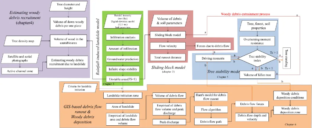
This study has three main goals: (1) to estimate the potential volume of woody debris due to rainfall-induced shallow landslides; (2) to study the entrainment process of woody debris due to debris flows; and (3) to evaluate the deposition zone of woody debris related to debris flows and shallow landslides. In order to achieve the study objectives, a research framework was conducted as presented in Figure 2.1. As mentioned in Chapter 1, the most significant cause of woody debris recruitment is landslides and debris flow processes, which act as a conveyor channelling woody debris downward from the hillslope or origin of the landslide. This study was divided into five main components: (1) a rainfall-induced shallow landslide model was developed to predict areas of instability which act a woody debris recruitment zones and debris flow initiation points; (2) a procedure was proposed for estimating potential woody debris recruitment caused by rainfall-induced shallow landslides; (3) to develop the sliding block model for debris flow runout; (4) the tree stability model was developed to evaluate the stability of trees related to debris flow forces; and (5) the woody debris deposition zone related to induced landslides and debris flows was evaluated using the integrated rainfall-induced shallow landslide and GIS-based debris flow runout models.

The rainfall-induced shallow landslide model allows for the assessment of shallow landslides triggered by rainfall. The rainfall-induced shallow landslide model combines two approaches: (1) a one-dimensional model of a rainfall-induced shallow landslide for predicting the time of occurrence of a shallow landslide and (2) a model for the simulation of rainfall-induced shallow landslides on a regional scale using a physically-based model, and a probabilistic approach for simulating shallow landslides caused by rainfall on a regional scale using a geographic information system platform. A detailed explanation of rainfall-induced shallow landslides is provided in Chapter 3.

The procedure for estimating woody debris recruitment caused by rainfall-induced shallow landslides uses areas of instability resulting from a model for the simulation of rainfall-induced shallow landslides on a regional scale using a physically-based model.

Satellite and aerial photographs provide the raw data for the estimations. Chapter 4 describes in more detail the process used to estimate woody debris recruitment due to rainfall-induced landslides.

The sliding block model for debris flow runout is a lumped mass model. The purpose

of the sliding block model is to explain the change in momentum due to woody debris entrainment. The sliding block model focuses on the transport process of debris flow. Chapter 5 provides a detailed explanation of the sliding block model.

The tree stability model explains the situation of trees in relation to the forces of debris flows. The tree stability model applies the concepts of root strength and the shear strength of soil. Chapter 5 describes in detail the concepts of root strength and the tree stability model.

The assessment of the deposition zone of woody debris is based on the grid system. Thus, Hunt’s model for debris flow runout and the conservation of mass equation are used to calculate debris velocity and debris flow depth. Moreover, the tree stability model is also used to evaluate tree stability. The conditions surrounding woody debris deposition and other relevant factors are explained in Chapter 6.

2.2 Data and sources

2.2.1 Digital elevation model

This study employed the digital elevation model (DEM), based on data from the ALOS-PALSAR, which was jointly built by the Japan Aerospace Exploration Agency (JAXA) and the United States National Aeronautics and Space Administration (NASA). The resolution of the ALOS-PALSAR DEM is approximately 12.5 meters.

2.2.2 Rainfall data

The rainfall data in this study were obtained from the Japan Meteorological Agency and the Thai Meteorological Department. The daily rainfall data were provided by the Japan Meteorological Agency and the Thai Meteorological Department.

2.2.3 Aerial photography

The aerial imagery obtained after a disaster provides critical data regarding landslides and debris flows scars in the target areas. In this study, aerial photographs of disaster-struck areas were obtained from the Geospatial Information Authority of Japan and NASA Earth Observatory, part of the EOS Project Science Office at the NASA Goddard Space Flight Center. 2.2.4 Global tree density map

The global tree density map provided the density of trees in the forest in the GeoTIFF files. The global tree density map was developed by Crowther et al. (2015) with the support of

17

the Yale Climate and Energy Institute and British Ecological Society. More than 420,000 ground surveys were conducted to estimate tree density around the world.

2.2.5 Soil types and depth of soil profiles

Soil types and depth of soil profiles were obtained from Version 3.1 of the ISRIC-WISE database. Version 3.1 of the ISRIC-ISRIC-WISE database provided the weight percentage of sand, silt and clay, which are the significant parameters used to classify the type of soil and to calculate the hydrological parameters, that is, the absolute depth to bedrock (Batjes 2009). In addition, soil samples were taken from the study sites to test the soil properties in the laboratory.

2.3 Field observation technique

Several parameters must be measured on site, such as the diameter and height of trees and the size of woody debris dams. Hence, this study measured certain parameters at the study sites for analysis.

2.3.1 Diameter and height of tree

The diameter of trees is a significant variable for assessing the potential volume of downed trees in this study. This study followed the Timber Cruising Handbook of the United States Forest Service. The diameter at breast height (DBH) of a tree represents the diameter of that tree. DBH was measured from the high ground side of the tree at 1.37 metres (4.5 feet) above the forest floor. A laser meter was used to measure the height of each tree.

2.3.2 Diameter and length of down tree

The method used to measure downed trees is also taken from the Timber Cruising

Handbook of the United States Forest Service. This measurement was also conducted using a

laser meter device.

2.3.3 Size of woody debris dam

Woody debris dams are one of the most important variables. It is necessary to calculate the volume of woody debris dams in order to validate the performance of the proposed model. This study measured the width, height and depth of woody debris at the study site. Furthermore, sketches of the shape of the woody debris were drawn.

18

CHAPTER 3

A MODEL TO ASSESS RAINFALL-INDUCED SHALLOW

LANDSLIDES

3.1 Introduction

Landslides are dangerous natural disasters which are described as the movement of surface material as a result of the force of gravity, and they normally occur on hillslopes and mountains (Dragicevic et al. 2015, Luo et al. 2015). Landslides occur mostly during rainy or typhoon seasons. The mechanism behind rainfall-induced shallow landslides is a rising water table, which builds significantly the positive pore water pressure on a slope. It may reduce the effective stress and leads to a reduction in shear strength on the failure plane. These changes may lead to shallow landslides or slope failure because the shear resistance in a hillslope is governed mainly by the shear strength of hillslope, in which effective stress is the main control parameter. Numerous studies have shown that the infiltration of rainwater play a key role in pore water pressure changes. Therefore, landslides are related to many factors, such as the ground water level, soil strength and infiltration process increasing the complications in modelling for landslides prediction. (Karam 2005, Rahardjo et al. 2008, Schnellmann et al. 2010, Zhang et al. 2011)

Therefore, the aim of this study is to develop a generalized model for shallow

landslides triggered by rainwater infiltration based on a deterministic model approach and GIS

spatial analysis while also considering the variance of soil parameters based on the simplified first-order second moment (SFOSM) method.

3.2 Theoretical background for shallow landslides triggered by rainwater infiltration

Based on the mechanism behindrainfall-induced shallow landslides, the deterministic

model used to analyse shallow landslides triggered by rainwater used in this study is based on two major hypotheses: 1) the shallow landslide characteristics are based on an infinite slope

and, (2) the hydrological conditions are based on steady state subsurface flow and the water

table is parallel to the topography. Hence, the deterministic model can be divided into three main parts: 1) rainwater seeps into the sloping soil surface, 2) the groundwater table generates caused by infiltrating rainwater and flows downslope, and 3) the stability of the slope changes in accordance with the groundwater level based on the limit equilibrium method.

19

3.2.1 Rainfall infiltration analysis

The Green-Ampt infiltration model is one of the most widely applied models and is used to calculate the infiltration rate and cumulative infiltration. The Green-Ampt infiltration model was first proposed for flow into an initially dry and uniform column of soil under ponded

infiltration conditions (Lu and Godt, 2013, Zhang et al. 2016). The Green-Ampt infiltration

model assumes that the soil suction head in the dry portion is constant and that the hydraulic conductivity and water content in the wet portion is also constant. Chen and Young (2006) extended the original Green-Ampt infiltration model to model a sloping surface. The infiltration rate and cumulative infiltration for the modified Green-Ampt equation for a sloping surface are presented in Equations 3.1 and 3.2 below.

 

 

 





_

_

where I(t) is the infiltration rate at time t (mm/day), i(t) is the cumulative infiltration at time t

(mm),  is the volumetric water content deficit









water content



k



k

cos



hydraulic coefficient (mm/day),



the slope angle (degree).

3.2.2 Analysis of the hillslope hydrologic process

A hillslope hydrology model is used to predict the steady groundwater table height. In the hydro-meteorological modelling framework, the recharge to groundwater is based on meteorological factors as follows (Sangrey et al. 1984):

R

 

P

Q

 

E

S



S

where R is the recharge of groundwater, P is the precipitation, Qr is the surface runoff, E is the

evapotranspiration, St is the storage, Sy is the synthetic elements. Considering the field situation,

evapotranspiration can be neglected during heavy or prolonged rainfall. Moreover, the storage and synthetic elements will be neglected for simplified calculation (Sangrey et al. 1984). The surface runoff is a consequence of the rainfall and infiltration processes.

Therefore:

20

where A is the contributing area (m2_{), I(t) is the infiltration rate at time t (m/day),}  _{is the}

soil porosity, m is the steady water table height (m), b is the width of the topographic element

(m), ky is the saturated hydraulic coefficient (m/day).

From Equation 3.4, the steady water table height can be expressed as follows:

 

3.2.3 Infinite slope stability model

The form of the failure plane for a shallow landslide is parallel to the slope surface and the depth of failure and length of failure are small. Therefore, the infinite slope stability model have been used widely for shallow landslide analysis. The infinite slope stability model employs factor of safety (FS). The FS is the ratio of the shear strength of the soil to the shear

stress required for equilibrium. If the value of factor of safety is less than 1.0, the slope is

unstable. It means that the shear strength is lower than the shear stress.

The factor of safety can be computed from the shear strength and shear stress of soils, can be expressed as follows:



 





 





















where c is the total cohesion (kPa),  is the friction angle of soil (degree). m is the

groundwater table height (m), D is the depth of soil (m), _satis the saturated unit weight of soil

(kN/m3),_tis the total unit weight of soil (kN/m3), where _wis the unit weight of water (kPa).

3.3 Simplified first-order second-moment method (SFOSM)

The simplified first-order second-moment method (SFOSM) is the probabilistic method used to estimate the probability of failure. The shear strength and shear stress are subjected to uncertainties that make the factor of safety uncertain, as well. The first-order second-moment method uses the first-order terms of a Taylor series to calculate the variance or second moment of the performance function. The distribution of random variables is represented by their mean and standard deviation. The probability density function of the random variables and the performance functions are assumed to have normal distributions. (Christian et al. 1994, Duncan 2000, Soralump 2002, Zhang et al. 2016)

The concept of this model is described as follows:

21

where FS is the factor of safety for infinite slope stability model, g( ) is the performance

function, xi is the soil properties and geometry, and e is the modelling error.

The expected value of performance variable (E[FS]):

E F S

 



     

 



where the performance function g(E[ ]) is calculated using input parameters that correspond to

the mean values of the component random variables, E[xi] is the mean valuesof the component

random variables.

The uncertainty in FS can be by its variances. These can be calculated by expanding the Equation 3.8 in the Taylor series and truncating to the first terms to yield:

 

 



where V[FS] is the variance operator, C(xi,xj) is the covariance of xi and xj and g( ) is the

performance function. In addition, C[xi,xj] = V[xi]

For the simplified First-order second-moment, the model error and spatial variability are neglected; hence, the Equation 3.9 can be rewritten as follows:

 

 



The standard deviation of factor of safety (



 

 

 

  (3.11)

The coefficient of variation of random variables can be calculated by using the following relationship.

 

 

22

Table 3.1 Coefficient of variation of parameters.

Parameters Coefficient of variation Reference

Soil cohesion 30% Baecher and Christian 2003

Slope angle 5% Karam 2005

Groundwater table 10% Karam 2005

Depth of soil 5% Karam 2005

Saturated unit weight of soil 3% Soralump 2002

Total unit weight of soil 10% Soralump 2002

Friction angle 15% Baecher and Christian 2003

Based on the assumption of SFOSM, the factor of safety is normally distributed and used to calculate the probability of failure and reliability index. Specifically, the mean and variance of factor of safety are used to compute the reliability index. Equation 3.13 represents the reliability index based on the normally distributed factor of safety. The probability of failure for the normally distributed factor of safety is shown in Equation 3.14 (Baecher and Christian 2003, Phoon and Ching 2014)

 

 







where



expected value of factor of safety,



 

the probability of failure.



theoretical fact that a normally distributed uncertainty on factor of safety gives a probability of failure of 0.5 at a factor of safety of 1 (Silva et. al. 2008), Hence, this study applies this condition for probabilistic analysis.

3.4 One-dimensional model of a rainfall-induced shallow landslide

The one-dimensional model of a rainfall-induced shallow landslide is proposed to estimate the time of occurrence of a shallow landslide. Figure 3.1 presents the computational flow chart for this one-dimensional model of a rainfall-induced shallow landslide.

23

Figure 3.1 Computational flow chart for one-dimensional model of rainfall-induced shallow landslide.

3.4.1 Description of studied areas

3.4.1.1 Iwaizumi landslide, Japan

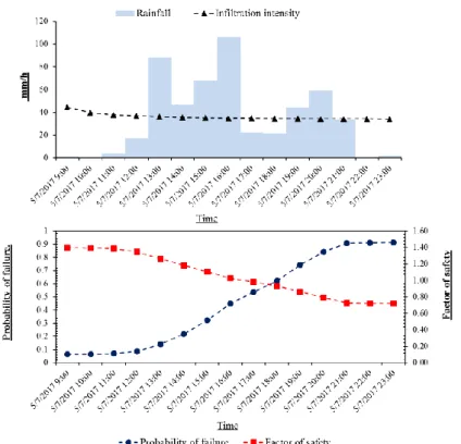
Typhoon Lionrock made landfall on the Pacific coast of north-eastern Japan on 30 August 2016. It brought heavy rainfall to the north-eastern region of Japan, causing landslides, debris flows, and floods. The accumulate rainfall at the Iwaizumi observation site was approximately 200 mm on 30 August 2016. During the 4 hours around when Typhoon

Lionrock passed through, the cumulative rainfall was approximately 160 mmat the Iwaizumi

(JMA) rain gauge operated by the Japan Meteorological Agency (JMA). The landslides occurred mostly on slopes ranging from 19 to 58 degrees. The depth of landslide scars was about 0.5-1.5 meters. Figure 3.2 presents the hourly rainfall and cumulative rainfall on 30 August 2016 at the Iwaizumi (JMA) rain gauge. (Chaithong et al, 2018)

Figure 3.2 Hourly rainfall and cumulative rainfall on 30 August 2016 at the Iwaizumi (JMA) rain gauge.

24

3.4.1.2 Asakura landslide, Japan

Tropical storm Nanmadol struck the island of Kyushu to the south of Japan on 4 July 2017. Nanmadol was third named tropical cyclone in 2017 and was Typhoon No. 1703. It had an effect on the cities on the island of Kyushu between 4 and 6 July 2017, especially the city of Asakura in Fukuoka prefecture of island Kyushu. The peak hourly rainfall measured by the Japan Meteorological Agency (JMA) at the Asakura rain gauge was 106 mm on 5 July 2017 at 16:00 p.m. The accumulate rainfall from was approximately 515 mm, more than a quarter of the average annual rainfall of 1,918 mm (as measured from 1976 to 2017) at the Asakura rain gauge. The landslide scars occurred mostly found on slopes ranging in angle from 20 to 50 degrees in the city of Asakura in Fukuoka prefecture. These Asakura scars made up approximately 67 % of the total landslide scars. Figure 3.3 presents the hourly and cumulative rainfall at the Asakura rain gauge during Nanmadol.

Figure 3.3 Hourly rainfall and cumulative rainfall on 5 July 2017 during 9:00 to 23:00 at the Asakura (JMA) rain gauge.

3.4.2 Results and discussion of the one-dimensional model for rainfall-induced shallow landslide

3.4.2.1 Iwaizumi landslide, Japan

The Iwaizumi landslide was investigated after Typhoon Lionrock passed through in 2016. Soil samples were collected and tested in the laboratory to discover the soil properties for landslide analysis. The properties of the soil for the Iwaizumi landslide analysis

are 10.8 kPa for the total cohesion, 29.7 degrees for the friction angle of the soil and 16.7 kN/m3

for the saturated unit weight of the soil. Moreover, the angle of the soil slope is assumed to be 34 degrees, the depth of residual soil is 3 metres deep, and the saturated hydraulic coefficient is 0.71 m/day.

25

According to the infiltration analysis, the rainfall intensity was lower than the infiltration rate in the first 16 hours of elapsed time of rainfall but after 4:00 PM on 30 August 2016, the rainfall intensity was higher than the infiltration rate until the end of the rainfall. Figure 3.4 presents the plots of hourly rainfall, infiltration rate, mean factor of safety, and probability of failure for the Iwaizumi landslide in Japan. Considering the plot of the mean factor of safety, it shows that the mean factor of safety decreased gradually in the first 16 hours. At 4 PM on 30 August 2016, the mean factor of safety began to decrease rapidly, reaching 1 at around 7 PM on 30 August 2016. When the mean factor of safety was less than 1, the cumulative rainfall was equal to approximately 200 mm. Regarding the plot of the probability of failure, it shows that the probability of failure was almost constant during the first 16 hours of the elapsed time of rainfall. The plot of the probability of failure increased rapidly at the same time that the mean factor of safety was decreased rapidly. Probability of failure exceeded 0.5 at around 7 PM.

Figure 3.4 Hourly rainfall, infiltration rate, mean factor of safety, and probability of failure for Iwaizumi landslide in Japan

3.4.2.2 Asakura landslide, Japan

The Asakura landslide was investigated after Tropical Storm Nanmadol passed through in 2017. The properties of the soil for the Asakura landslide analysis are 12.7

kPa for the total cohesion, 24.8 degrees for the friction angle of the soil and 17.1 kN/m3 for the

26

the depth of the residual soil is 2.5 metres deep and the saturated hydraulic coefficient is 0.96 m/day.

Figure 3.5 presents the plots of the hourly rainfall, infiltration rate, mean factor of safety, and probability of failure for the Asakura landslide in Japan. According to the infiltration analysis, there are two periods in which the rainfall intensity was higher than the infiltration rate: from 1 PM to 4 PM on 5 July 2017 and from 7 PM to 8 PM on 5 July 2017. Considering the plot of mean factor of safety, it shows that the mean factor of safety was decreasing gradually with the elapsed time of rainfall. It deceased from approximately 1.4 at beginning of the rainfall to approximately 0.7 at the end of the rainfall. The mean factor of safety was less than 1 around 4 PM on 5 July 2017. The accumulate rainfall at the time that the mean factor of safety dipped below 1 was 332 mm. In regards to the trend in the probability of failure, it increased gradually from approximately 0.1 at beginning of the rainfall to

approximately 0.9 at the end of the rainfall.The probability of failure exceeded 0.5 for the first

time around 4 PM on 5 July 2017.

Figure 3.5 Hourly rainfall, infiltration rate, mean factor of safety, and probability of failure for Asakura landslide in Japan

27

3.5 A model for the simulation of rainfall-induced shallow landslides on a regional scale using a physically-based model and probabilistic approach

In this section, a model for predicting shallow landslide triggered by rainfall using a physically-based model and probabilistic approach is proposed. The purpose of the proposed model is to simulate shallow landslides caused by rainfall on a regional scale using a geographic information system platform. Figure 3.6 presents the calculation framework for the proposed model.

Figure 3.6 Calculation framework for the proposed model

The model’s prediction capability was verified by comparing the results from the actual shallow landslide cases in Thailand and Japan with the results of the proposed model. The receiver operating characteristic (ROC) curve is applied to evaluate the performance of the proposed model. There are four possible types of outcome when comparing the predicted result and the actual landslide: 1) true positive (TP), which means that the actual landslide grids are predicted as unstable grids; 2) false positive (FP), which means that the actual stable grids are predicted as unstable grids; 3) false negative (FN), which means that the actual landslide grids are predicted as stable grids, and 4) true negative (TN), which means that the actual stable grids are predicted as stable grids. (Zhang et al. 2016, Chaithong and Komori 2017)

The performance indices can be obtained using the confusion matrix.The true positive

rate can be calculated using Equation 3.15, the false positive rate can be computed using Equation 3.16, and the accuracy can be calculated using Equation 3.17.

True positive rate = TP

28

False positive rate = FP

N (3.16)

Accuracy = TP TN

P N



 (3.17)

where P is the condition positive (P = TP+FN) and N is the condition negative (N = TN+FP). 3.5.1 Results and discussion of a model for the simulation of rainfall-induced shallow landslides on a regional scale using a physically-based model and probabilistic approach

Iwaizumi landslide

The Iwaizumi landslide was also used to evaluate the performance of the proposed model. The details of the Iwaizumi landslide were given in Section 3.4.1.1. The soil properties used in the Iwaizumi landslide analysis are 10.8 kPa for the total cohesion, 29.7

degrees for the friction angle of the soil and 16.7 kN/m3 for the saturated unit weight of the

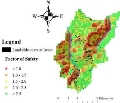
soil. Moreover, the saturated hydraulic coefficient is 0.72 m/day. Figure 3.7 presents the distribution of the cumulative rainfall for the Iwaizumi landslide analysis on 30 August 2016. The distributed rainfall was generated using five rain gauges in the town of Iwaizumi, Iwate prefecture, which were operated by operated by the Japan Meteorological Agency (JMA) and Iwate prefecture. To generate a rainfall distribution in this study, the inverse distance weighted interpolation method (IDW) in the Spatial Analyst Tool from ArcGIS was utilized. The maximum rainfall was approximately 203 mm and the minimum rainfall was approximately 194 mm. The localization of these landslide scars were obtained from the aerial photography provided by the Geospatial Information Authority of Japan after Typhoon Lionrock passed though the affected areas. Figure 3.8 presents the landslide scars and elevation data used in the

Iwaizumi landslide analysis.The elevation data were obtained from the ALOS PALSAR DEM

12.5 m, collaboratively developed by the National Aeronautics and Space Administration (NASA) and the Japan Aerospace Exploration Agency (JAXA). The slope angle was obtained from the 12.5-meter resolution ALOS PALSAR DEM using the Spatial Analyst Tool from ArcGIS.

29

Figure 3.7 Distribution of cumulative rainfall of the Iwaizumi landslide analysis on 30 August 2016

Figure 3.8 landslide scars and elevation data of Iwaizumi landslide analysis

Following the same criteria as in the Khao Panom landslide analysis, the factor of safety and probability of failure calculations show that the predicted unstable grids

(FS<1 and pf > 0.5) appear mostly on the high slope gradient areas. This result is in quite good

agreement with the landslide scars obtained via aerial photography. Figure 3.9 presents the factor of safety map for the Iwaizumi landslide analysis. Figure 3.10 presents the probability of failure map for the Iwaizumi landslide analysis. Considering the accuracy of the proposed

30

model, it shows that the accuracy of the factor of safety map is approximately 0.84 and the accuracy of the probability of failure map is approximately 0.84. Figure 3.11 presents the ROC curves for the factor of safety and probability maps and both ROC curves appeared above of the random guess line, indicating that the proposed model exhibits a good performance in landslide prediction. The area under ROC curve for the factor of safety map is 0.72 and the area under ROC curve for the probability of failure map is 0.71. Comparing the maps there is a small difference between their results.

Figure 3.9 Factor of safety map of Iwaizumi landslide analysis

Figure 3.10 Probability of failure map of Iwaizumi landslide analysis

31

Figure 3.11 Receiver operating characteristic curve of factor of safety and probability maps of Iwaizumi landslide analysis

3.6 Conclusion

The aim of this study was to develop models that can predict the occurrence of shallow landslides triggered by rainwater infiltration. The models were divided into 2 types of approaches: a one-dimensional model for rainfall-induced shallow landslides and a model for simulating rainfall-induced shallow landslides on a regional scale using a physically-based model and probabilistic approach. The proposed one-dimensional model for rainfall-induced shallow landslides was used to estimate the times of occurrence for shallow landslides. Considering the results of the model, it can predict the timing of shallow landslides well. The predicted results and actual observations were in good agreement. The model used to simulate rainfall-induced shallow landslides on a regional scale aimed to predict the locations of unstable areas using the GIS approach. The model can predict slope instability zones and there is the good correspondence between the predicted unstable zones and actual landslide scars. The Iwaizumi landslide case, the accuracy is 0.72 for the model based on factor of safety and 0.71 for the model based on the probability of failure. The results of these cases demonstrate that this physically-based model has the potential to become a practical method for assessing landslide hazards on a regional scale.

32

CHAPTER 4

ESTIMATING WOODY DEBRIS RECRUITMENT IN A STREAM

CAUSED BY A TYPHOON-INDUCED LANDSLIDE: A CASE STUDY

OF TYPHOON LIONROCK IN IWAIZUMI, IWATE PREFECTURE,

JAPAN

4.1 Introduction

When landslides occur, the slope movement disturbs tree roots, causing the trees to topple. The fallen trees become woody debris, some of which remains upslope and some of which is entrained by debris flows or flash floods that flow downstream (Phien-wej et al. 1993, Montgomery and Buffington 1993, Chaithong et al. 2018a, Chaithong et al. 2018b).

On 30 August 2016, Typhoon Lionrock made landfall on the Pacific coast of northeast Japan (Tohoku region). The typhoon caused flash floods, landslides and debris flows throughout the Tōhoku region. Typhoon Lionrock brought heavy rainfall, reaching a maximum hourly rainfall of 66 mm at the Iwaizumi (JMA) rain gauge. Vast quantities of woody and other debris were observed in the town of Iwaizumi, Iwate Prefecture, in Japan’s Tohoku region. Figure 4.1 illustrates the woody debris deposited in the town of Iwaizumi, Iwate prefecture, in the northeast of Japan. Based on the results of this investigation, landslides are a significant generator of woody debris, which is subsequently entrained by debris flows. Therefore, the aim of this study was to develop a procedure for estimating woody debris recruitment into streams following landslides.

33

4.2 Description of the study site

The study area is a sub-watershed in the Omoto river basin located in the town of Iwaizumi, in Japan’s Iwate Prefecture. The total length of the channel is approximately 3.75

km and the area of the sub-watershed is approximately 0.87 km2_{. The study site is used as an}

artificial forest, in which the main tree species are Hinoki (Chamaecyparis obtusa) and Sugi (Cryptomeria japonica). The post-disaster investigation showed that the woody debris blocked a dam in a narrow downstream section. The total volume of the woody debris dam in the narrow

downstream section was approximately 524 m3 _{(including voids). The total volume of woody}

debris dams in the upstream part of the study site was approximately 668.5 m3 _{(including voids).}

The volume of woody debris in the dam located in the stream channel in the upstream area of

the study site was approximately 178 m3 (including voids), while that in the dam located on

the hillslope was approximately 490.5 m3 (including voids). As for the characteristics of woody

debris pieces in the narrow downstream section, the mean length of the woody debris pieces was 5.2 ± 4.8 m, and the mean diameter of woody debris pieces was 0.22 ± 0.1 m. Moreover, the woody debris dams in the upstream part of the study area had a mean height of 2.7 ± 1.6 m, a mean width of 5.9 ± 2.8 m, and a mean depth of 4.7 ± 2.5 m.

4.3 Methods and dataset

The proposed procedure can be divided into the following four steps:

a) The first step involves simulating the areas of instability (landslide areas) with an analytical rainfall-induced shallow landslide model that describes the source of woody debris recruitment to the watershed.

b) The second step is performing a forest analysis to determine tree diameter, tree height and tree density, as well as estimating the volume per piece of downed woody debris. c) The third step is using satellite images and aerial photographs to identify the width of

the active stream channel following the debris flow.

d) In the final step, the parameters – the areas of instability, the volume per piece of downed woody debris, the tree density, and the width of the active stream channel – are used to estimate woody debris recruitment into the stream channel caused by landslides induced by Typhoon Lionrock. To estimate woody debris recruitment, I calculate the volume of woody debris in the area of overlap between the unstable area and the active channel area, assuming that only woody debris in the active channel zone could be entrained into the stream channel, based on the work of Mazzorana (2009) and Lange (2016).

The performance of this procedure will be validated by comparing the amount of woody debris estimated using the proposed procedure and the total amount of woody debris in the stream and damming a narrow downstream section, as determined during a field survey of the study site.

34

Figure 4.2 presents the procedure for estimating woody debris due to rainfall-induced shallow landslides. Table 4.1 presents the parameters for the estimation of woody debris recruitment.

Figure 4.2 Procedure for estimating woody debris due to rainfall-induced shallow landslide Table 4.1 Parameters for the woody debris recruitment estimation

Parameters Unit Value

Total cohesion kPa 10.8

Friction angle degree 29.7

Saturated unit weight of soil kN/m3 _16.7

Unit weight of water kN/m3 _9.81

Hydraulic conductivity m/day 0.72

Porosity of soil - 0.437

Suction at wetting front mm 61.3

Volumetric water content deficit - 0.27

4.4 Results and discussion

Huber’s formula was modified to calculate the potential volume of downed woody debris. The values of tree height at the study site showed that the minimum tree height was approximately 5 m, while the maximum tree height was approximately 25 m; therefore, the tree height and diameter data sets were treated as uncertain variables in the modified Huber formula. Hence, in this study, Monte Carlo methods (MCMs) were used to estimate the volume of downed woody debris. The values for each parameter were generated using random and independent but non-identical distributions; each parameter generated 10,000 random values. The peak of the distribution curve for the volume of downed woody debris, which is

35

Table 4.2 presents the results for woody debris recruitment caused by the Typhoon Lionrock–induced landslide. The field survey revealed woody debris dams along the stream channel and on hillslopes. The volume of woody debris dams located in the stream channel in

the upstream part of the study site was approximately 178 m3 (including voids), while the

volume of the woody debris dam located on the hillslope was approximately 490.5 m3

(including voids). The total volume of the woody debris dam in the narrow downstream section

was approximately 524 m3 (including voids). Based on the assumption that only woody debris

in the active channel zone could be entrained into the stream channel, as suggested by Mazzorana (2009) and Lange (2016), the volume of woody debris in the stream caused by the

Typhoon Lionrock–induced landslide was 702 m3. According to my calculations, potential

woody debris recruitment into the active channel was approximately 638 m3. Therefore, the

model proposed in this study underestimated the woody debris entrained downstream by approximately 9%.

Table 4.2 Results for woody debris recruitment caused by the Typhoon Lionrock-induced landslide

Unit Values

Un Unstable area (FS<1) km2 0.42

Potential volume of fallen tree in the unstable area trees 25,350

Potential woody debris recruitment in the unstable area m3 _19,010

Woody debris recruitment in active channel m3 ₆₃₈

4.5 Conclusion

This study developed a procedure for estimating the recruitment of woody debris downstream. The proposed procedure can estimate potential woody debris recruitment; however, the procedure underestimates this amount compared to field-based measurements.

36

CHAPTER 5

A MODEL FOR ASSESSMENT OF TREE STABILITY AND

ENTRAINMENT OF WOODY DEBRIS BY FLOW SLIDES AND

SHALLOW SLOPE FAILURE

5.1 Introduction

Shallow landslides and flow slides overturn, uproot and break trees. Debris flows can demolish objects on the flow route. When trees overturn, the root clusters and surrounding soil are uprooted together. In relation to uprooted trees, the failure mode of overturning trees can take one of two forms: shear failure of soil and soil–root failure. The shear failure of soil is a slide along the slip plane without any root resistance. The soil–root failure mode is a soil failure in the presence of root resistance. The soil–root failure mode is characterised by the failure plane passing through both the soil and the root of the tree in a semicircle or part-circle in two dimensions – that is, in the shape of a half-cylinder and a hemisphere (Bartelt and Stöckli 2001, Rahardjo et al. 2009, Rahardjo et al. 2017).

Therefore, this study proposes a model to describe the mechanism of tree instability caused by shallow slope failures and flow slides, including the entrainment of woody debris by flow slides or debris flows.

5.2 Description of rainfall-induced shallow landslide model, sliding block model and tree stability model

5.2.1 Rainfall-induced shallow landslide model

The rainfall-induced shallow landslide model is described in detail in Chapter 3. Coppin and Richards (1990) proposed that the main influences of trees on the stability of the hillslope can be included in the factor of safety equation in terms of root cohesion. Therefore, Equation 3.6 was modified, and Equation 5.1 includes the modified safety factor:



 

























37

In addition, Kondo et al (2004) proposed the equation provides the root cohesion (cr).

782 0 . 5 5

r r

c    k



where



Equation 5.4, and dr is the diameter of root of Japanese cedars (m).



k 











In this study, the mobilisation hypothesis of the sliding block model is based on Iverson’s (1997) concept. The sliding block model is a lumped mass model utilised to describe

the movement of the centroid of a debris flow.The debris flow begins to accelerate when the

acting force exceeds the movement resistance force caused by the frictional force. Therefore, to analyse sliding block motion, the acting force is a significant result of the driving force and movement resistance. In this analysis, gravity imposes a driving force, while the movement resistance is developed based on a combination of Coulomb’s friction law and Terzaghi’s effective stress principle. The sum of the driving force and movement resistance is the net force, as shown in Equation 5.5.

F_n  M_d  G















where Fn is the net force (kN*m/s2), Md is the mass of debris flow (kN), G is the gravitational

acceleration (m/s2), ru is the pore pressure ratio.

In terms of the mass of debris flows, there are two main phases: solid and liquid. Generally, soil and rock are the main components of the solid phase. The mass of the debris

flow (Md) can be calculated using Equation 5.6:

M

 



V

38

Thus, the mass of the debris flow after the entrainment process can be calculated using Equation 5.7:

M





V





V

where



that is entrained by the debris flow (m3).

The velocity in each time step can be calculated using:

_{i 1 i} n i d F t mv v v M       (5.8)

where vi+1 is the velocity at time i+1 (m/s) and vi is the velocity at time i (m/s).

The displacement of the slide block can be calculated by Equation 5.9:

s_i1 s_i 0.5t v





where si+1 is the displacement at time i+1 (m), and si is the displacement at time i (m). Figure

5.1 presents schematic of motion of debris flow in time step and woody material entrainment.

Figure 5.1 Motion of debris flow in time step and woody material entrainment

Considering the attack between debris flow and tree, three main types of force— namely hydrostatic, impact, and drag forces—assail trees as a consequence of debris flow. These are considered as shown below. (He et al. 2016, Gao et al. 2017)

39

F_{i m}



F



0 . 5



v H D C

where Fhs is the hydrostatic force (kN). Hd is the depth of debris flow (m). Dt is the diameter

of tree at breast height (m). Fim is the impact force (kN). is the impact force coefficient

which Canelli et al. 2012 recommended the impact force coefficient is 1.5-5.5. Fdr is the drag

force (kN). CD is the drag coefficient.

5.2.3 Tree stability model

Based on our observations, the mode of tree failure is assumed to be a soil–root failure mode. Figure 5.2 shows the roots of Hinoki after tree failure. In this study, the case of the hemisphere shape was considered because the hemisphere shape is in good agreement with the observational data and the assumed distribution of cedar tree roots proposed by Kondo et al. (2004, 2007). Moreover, the concept of shear strength is based on the Mohr–Coulomb failure criterion. Figure 5.3 provides a schematic representation of the tree stability analysis. The stability of the tree is the ratio of the resisting shear force to the driving shear force, as shown in Equation 5.13.

40

Figure 5.3 Schematic of tree stability analysis and distribution of flow slide forces

m s r m t h s h s i m i m d r d r R Ts R W F R F R F R



where Ts is the tree stability index.



moment arm of total shear strength of tree (m). Wt is total weight that is the summing weight

of tree and weight of soil (kN). Rhs is the moment arm of hydrostatic force (m). Rim is the

moment arm of impact force (m). Rdr is the moment arm of drag force (m). The shear strength

on the slip surface is represented by Equation 5.14.





where



summation of soil cohesion and root cohesion (c+ cr), r is the radius of hemisphere (m), m is

the height of water table (m).

Considering to the driving force, the total weight can be calculated using Equation 5.15.















where Vtree is the volume of tree (m3).

For simplified calculation, I assume that the centre of overturning is the centroid of

the hemisphere in the initial moment of tree failure. Therefore, the moment arm of the total shear strength of the tree can be calculated as follows: