Models in Microbial Ecology and Related Problems in Ordinary and Partial Differential Equations(Mathematical Topics in Biology)

Models

in

Microbial

Ecology and Related Problems

in Ordinary

and Partial

Differential

Equations

Sze-Bi

Hsu

Institute of Applied Mathematics, National Tsing-Hua University,

Hsin-chu, Taiwan

Abstract. In this article, we survey the mathematical models of severval microorganisms

compet-ing for a scompet-ingle-limited nutrient. Several mathematical models in the form of system ofordinary

differential equations or partial differential equations arepresented to explain the competitive

ex-clusion and the coexistence of the species.

1

Introduction

Human being cannot survive without microorganisms. It is important to understand the

ecological behavior of microorganisms in their communities, for example, the competition,

predation, mutualism, inhibition effects [FS]. In thispaper, we shall restrict our attentitions

to the mathematical models ofseveral microorganisms competing for a single-limited

nutri-ent. For the case of multiple nutrients, interested readers may consult [CHH], [WHH]. There

are several reasons to study these mathematical models. Firstly,we have different ecological

view points about the validity of the classical Lotka-Volterra two species competition model

$\neq=\gamma_{1}x_{1}(1-\neq)-\alpha_{1}x_{1}x_{2}dx_{t}x_{1}$

(1.1) $\neq_{t}^{dx}=\gamma_{2}x_{2}(1-\neq^{x_{2}})-\alpha_{2}x_{1}x_{2}$,

$x_{1}(0)>0$, $x_{2}(0)>0$

Gauss (1934) used bacteria to verify the validity of the model [H]. However the competition

coefficients $\alpha_{1},$ $\alpha_{2}$ are not “physical” parameters which cannot be measured in advance of

type interaction, coupled with the type2 functionalresponse, to construct our mathematical

models where the parameters can be measured in advanced of the experiments. Secondly,

the models are also relatedto theecology of lakes andstreams. Weshall present the

“chemo-stat” equation. Chemostat is an laboratory apparatus where both theory and experiments

are tractable and match. Thirdly in the application to Chemical engineering, the industrial

microorganisms are used to “eat” the industrial waste water [PC], [SFA]. Chemostat is also

used to culturethe usefulindustrial microorganisms. Andfinally, thereare interesting

math-ematical problems in these mathematical models, for example, global stability, uniqueness of limit cycle, periodic solutions, persistent theory in dynamical system, strongly monotone flows.

2

Simple Chemostat (Well-Stirred)

The chemostat is a piece of laboratory apparatus used for culturing microorganisms. It

has a constant nutrient source, containing all nutrients needed by the microorganisms in

aboundance except one. The nutrient is pumped at a constant rate into a culture vessel.

Constant

volume is maintained in the culture vessel by allowing an overflow or by pumping

the contents of vessel out at the same rate that nutrient is pumped in. The output of the

culture vessel is collected in a receptacle. The culture vessel is charged with a quantity of

a given type of microorganism and the collection vessel then contains both organisms and

nutrient. This provides a continuous supply of microorganisms. For ecological purpose the

chemostat is the laboratory realization of a very simple lake; the importance of the

chemo-stat as an experimental vehicle is well documented [FS], [V], [P]. It is also of interesting in

chemicalengineering where it is a simplified model ofthewastewater treatment process [PC].

Based on the experimental evidence [Mo], we assumed

(i) The growth rate of a microorganism species obeys the Michaelis-Menten kinetics, i.e.

$\frac{1}{x}\frac{dx}{dt}=\frac{mS}{a+S}$

Where $S$ is the concentration of the nutrient, _$m$ is the maximum growth rate and _$a$ is

the half-saturation constant.

(ii) The growth can be expressed in terms of the nutrient consumed by

Where $y$ is a yield constant expressed as

$y= \frac{organismformed}{substrateused}$

For simplicity, we consider thecase of two species. Then chemostat equation takes theform

$\mathcal{T}tdS=(S^{(0)}-S)D_{1}-\frac{m}{y}1\frac{S}{a_{1}+S}x_{1_{2}^{-\frac{m}{y}4_{\frac{S}{a_{2}+}}}}F^{X_{2}}$ $\neq^{dx_{l}}=(\frac{m_{1}S}{a_{1}+S}-D)x_{1}$ (2.1) $\neq^{dx_{l}}=(\frac{m_{2}S}{a_{2}+S}-D)x_{2}$ $S(O)\geq 0$, $x_{1}(0)>0$, $x_{2}(0)>0$ where

$S(t)=the$ concentration of nutrient at time $t$

$x;(t)=the$ concentration of i-th micororganism at time $t$

$S^{\langle 0)}=input$ concentration ofthe nutrient

$q=flow$ rate

$V=volume$ of the vessel

$D=\theta=dilution$ rate

We note that the parameters $S^{(0)}$ and

$q$ are controlled by the experimenter.

For system (2.1) our basic assumption is

where

$\lambda_{i}=\frac{a_{t}D}{m_{i}-D}$ is the “break-even” concentration for i-th species

Theorem [HHWI], [Hsul]

Let (H) hold. Then the solution of (2.1) satisfy

$\lim_{tarrow\infty}S(t)=\lambda_{1},\lim_{tarrow\infty}x_{1}(t)=x_{1}^{*}>0,\lim_{tarrow\infty}x_{2}(t)=0$

Remark: Species with smallest $\lambda$ wins the competition. Smaller half-saturationor larger

maximum growth rate implies smaller A.

Sketch of the Proof:

Construct the following Liapunov function

$V(S, x_{1}, x_{2})= \int_{\lambda_{1}}^{s}\frac{\xi-\lambda_{1}}{\xi}d\xi+c_{1}\int_{xi}^{x_{1}}\frac{\xi-xi}{\xi}d\xi+c_{2}x_{2}$

for some $c_{1}>0_{\}}c_{2}>0$. Applying LaSalle’s invariance principle completes the proof.

Remark : Recently Wolkowicz&Lu [WL] construct a new Liapunov function for general

functional responses.

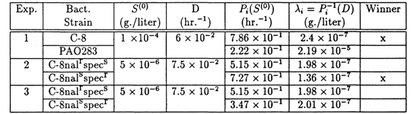
The best known series of laboratory experiments preformedfor thepurpose oftestingthe

validity of the chemostat equation werecarriedout by Hansen and Hubbell [HH].A summary

of their experiments is given in Table below. The parameters of the model were measured

by growing each of the competitors separately on the growth-limiting nutrient tryptophan

and assuming Michaelis-Menten functional responses. In Experiment 1,

C-8

is a particular

strain of Escherichia coli and

PAO283

isastrain of Psuedomonas aeruginosa. In Experiment

2, the competition was between two variants of C-8, one which is resistant to the inhibitor

naladixic acid but susceptible to spectinomycin, and the other the reverse. In both of these

experiments, the species predicted to win by the model did indeed win even though it

was

originally inoculated into the growth vessel in a much smaller amount than the predictd

los-er. In the third experiment, the C-8 variants were used again, but naladixic acid was added

to the culture medium in the proper amount so that the parameters $\lambda_{i}=P_{1}^{-1}(D),$$i=1,2$

coexist in the growth vessel for as long as the experiment was run (120 hours).

Table 5.1 Summary ofHansen-Hubbell experiments

Inspired by the Hansen-Hubbell experiment, Lenski and Hattingh [LH] construct the

fol-lowing model describing the competition in a chemostat with external inhibitor. Let $P(t)$

be the concentration of external inhibitor, for example, pollutant or antibody. We

assume

the species 1 is susceptible to the inhibitor while the species 2 is resistant. Only species 2

consumes the inhibitor. Then the equations takes the form

$\mathcal{T}tdS=(S^{(0)}-S)D-\frac{m_{1}S}{a_{1}+b}x_{1}e^{-\lambda P}-\frac{m_{2}S}{a_{2}+b}x_{2}$

$\neq^{dx}t=(\frac{m_{1}S}{a_{1}+S}e^{-\lambda P}-D)x_{1}$

(2.2) $\neq^{dx}t=(\frac{m_{2}S}{a_{2}+S}-D)x_{2}$

$-\tau tdP\delta xP=(P^{\langle 0)}-P)D-\iota\neq+T$

$S(0)\geq 0,$ $x_{1}(0)>0$, $x_{2}(0)>0,$ $P(O)\geq 0$,

Where $P^{(0)}$ is the input concentration of the inhibitor.

In $[HsW1]$ the authors observed that the solution of (2.2) satisfies $S(t)+x_{1}(t)+x_{2}(t)=S^{(0)}+O(e^{-Dt})$ as $tarrow\infty$

$\neq_{t}^{dx}=(\frac{m_{1}(S^{(0)}-x_{1}-x_{2})}{a_{1}+(S^{(0)}-x_{1}-x_{2})}e^{-\lambda P}-D)x_{1}$

(2.3)

$\neq_{t}^{dx}=(\frac{m_{2}(S^{\{0)}-x_{1}-x_{2})}{a_{2}+(S^{(0)}-x_{1}-x_{2})}-D)x_{2}$

$\underline{d}P\delta x_{+}P\tau_{t}^{=(P^{(0)}-P)D-\infty}$

$0<x_{1}(0)+x_{2}(0)<S^{\langle 0)},$ $P(0)\geq 0$

.

Since (2.3) is a competitive system in $R^{3}$, from [Hir], [Sm3] we have Poincar\’e-Bendixson

Theorem. When the interior equilibrium $E_{c}=(xi,x_{2}, P)$ exists , we show that for large

$\lambda,$$\delta$ and small $K,$_{$E_{c}$} is unstable. Thus the coexistence occurs in the form of periodic

solutions

3

Coexistence

In this section we shall search for possible reasons for coexistence which is aften observed in

the nature.

I.

Assume $S$ is the prey which grows logistically. Consider the following “model” equation

first studied by Koch [Ko] and then analyzed in [HHW3]

$7^{\frac{S}{t}}d=rS(1_{K}^{S}-)- \frac{m_{1}S}{a_{1}+S}x_{1}-\frac{m}{a_{2}}+Ls_{F^{X_{2}}}$

$\neq^{dx}t=(\frac{m_{1}S}{a_{1}+S}-D_{1})x_{1}$

(3.1)

$\neq^{dx}t=(\frac{m_{2}S}{a_{2}+S}-D_{2})x_{2}$

$S(O)>0,$ $x_{1}(0)>0,$ $x_{2}(0)>0$

(H1) $0<\lambda_{1}<K$, $\lambda;=\frac{a_{i}D_{:}}{m_{1}-D:}$, $i=1,2$

Theorem

3.1

: (Extinction) Let (H1) hold and $b_{i}= \frac{m:}{D_{:}}$

,

$i=1,2$

.

If

(3.2) $a_{1}<a_{2}$, $b_{1}>b_{2}$ or

(3.3) $a_{1}<a_{2}$

,

$b_{1}<b_{2},$ $K< \frac{b_{1}a_{2}-b_{2}a_{1}}{b_{2}-b_{1}}$

then $\lim_{tarrow\infty}x_{2}(t)=0$

To understand the dynamics of (3.1), we need to study the two-dimensional Predator-Prey

system.

$7^{\frac{S}{t}=\gamma S(1-}K^{)-\frac{mS}{a+}}F^{x}dS$

(3.4) $Tt+T^{-D)x}d_{X_{-=(\frac{m}{a}}}S$

$S(O)>0,$ $x(O)>0$

Theorem 3.2 : Let $0<\lambda<K,$ $\lambda=\frac{aD}{m-D}$

.

(i) If$\frac{K-a}{2}\leq\lambda$ then the solution _$S(t),$ $x(t)$ of (3.4) satisfy

$\lim_{tarrow\infty}S(t)=\lambda$, $\lim_{tarrow\infty}x(t)=x^{*}>0$

(ii) If$\frac{K-a}{2}>\lambda$, then there exists a unique limit cycle.

Insterested readermayfind the proof of(i) in [HHW3] and that of(ii) in [Ch].

Condiser

our

one prey-two predators system (3.1), we have the following

extinction

results.

Theorem 3.2: Let (H1) holdand either(3.2) or (3.3) hold. Then the solution $\{S(t),x_{1}(t),x_{2}(t))$

of (3.1) satisfies.

$\lim_{\ellarrow\infty}S(t)=\lambda_{1}$

$\lim_{\ellarrow\infty}x_{1}(t)=x_{1}^{*}>0$

$\lim_{tarrow\infty}x_{2}(t)=0$

(ii) If$\frac{K-a_{1}}{2}>\lambda_{1}$ then the trajectory $(S(t)\cdot x_{1}(t), x_{2}(t))$ approach the unique limit

cycle $\Gamma_{1}$ in $S-x_{1}$ plane except the one dimensional stable manifold of $(\lambda_{1}, x_{1}^{*},0)$

In [HHW2], the numerical studies shows that under the assumption $0<\lambda_{1}<\lambda_{2}<K,$ $a_{1}<$

$a_{2},$ $b_{1}<b_{2},$ $K>rightarrow^{ba_{2}-b_{1}ab-b}$, varying $K$ from $\infty ba_{2}-b_{1}ab-b$ to infinity produces a family of

positive periodic solutions emerging from $\Gamma_{1}$ and decending to $\Gamma_{2}$

.

Recently [MR] Murator

assume the parameter $\gamma$ is large and apply the singular pertubation technique to justify

the phenomena. Butler and Waltman [BW] apply the result in [Ch] to show that when $\Gamma_{1}$

becomes unstable, there is a familyof positive periodic solutions bifurcating from $\Gamma_{1}$

.

Smith

[Sm2] also shows the existence of positive solution by Hopf bufurcation. Next we consider

one nutrient-one prey-twopredatorsin the chemostat. The equations take thefollowing form.

$dSTt=(S^{(0)}-S)D- \frac{m_{1}S}{a_{1}+S}x$

$- \tau tdx=(\frac{m_{1}S}{a_{1}+S}-D-\frac{m_{2}y}{a_{2}+x}-\frac{m_{3}z}{a_{3}+x})x$

(3.5) _{$\neq_{t}^{d}=(\frac{m_{2}x}{a_{2}+x}-D)y$}

$7^{\frac{z}{t}}d=( \frac{m_{3}x}{a_{3}+x}-D)z$

$S(O)\geq 0,$ $x(O)>0,$ $y(O)>0,$ $z(O)>0$

The behavior of solutions of (3.5) is similar to that of (3.1). Interested reader may consult

[BHWI]

$\Pi$

.

Periodic input and periodic washout rate when the imput concentration is a periodic

$dSTt=( \varphi(t)-S)-\frac{m_{1}S}{a_{1}+S}x_{1}-\frac{m_{2}S}{a_{2}+S}x_{2}$

$\neq^{dx}t=(\frac{m_{1}S}{a_{1}+S}-D)x_{1}$

(3.6)

$\neq^{dx}t=(\frac{m_{2}S}{a_{2}+S}-D)x_{2}$

$S(O)>0,$ $x_{1}(0)>0,$ $x_{2}(0)>0$

In [Hsu2], we study the extinction, persistence of the solutions of (3.6) for the special case

$\varphi(t)=S^{(0)}+b\sin\omega t$

.

A numerical study shows thecoexistence ispossible in the b-w

param-eter region. Smith [Sml] shows the existence of $\frac{2\pi}{w}$periodic solutions by Hopf bifurcation

Hale and Somolinas $[HaS]$ observe the relationship $S(t)+x_{1}(t)+x_{2}(t)=\Phi(t)+o(e^{-\alpha\ell}),$ $\alpha>$

$0,$ _{$\Phi(t+w)=\Phi(t)$} and reduce the dynamics of (3.6) to a competitive, periodic two

dimen-sional system

$\neq^{dx_{l}}=(\frac{m_{1}(\Phi(t)-x_{1}-x_{2})}{a_{1}+(\Phi(t)-x_{1}-x_{2})}-D)x_{1}$

(3.7)

$\neq^{dx}t=(\frac{m_{2}(\Phi(t)-x_{1}-x_{2})}{a_{2}+(\Phi(t)-x_{1}-x_{2})}-D)x_{2}$

and apply the results obtained by de Mottoni and Schiaffino [MS] which states any solution

of two-dimensional, periodic, competitive system approaches to a periodic solution. For the

appliction to industrial waste water in Chemical Engineering, the dilution rate is periodic.

$- \tau tdS=(S^{\langle 0)}-S)D(t)-\frac{m_{1}S}{a_{1}+b}x_{1}-\frac{m_{2}S}{a_{2}+S}x_{2}$

$\neq^{dx}t=(\frac{m_{1}S}{a_{1}+b}-D(t))x_{1}$

(3.8)

$\neq^{dx_{l}}=(\frac{m_{2}S}{a_{2}+S}-D(t))x_{2}$

$S(O)\geq 0,$ $x_{1}(0)>0,$ $x_{2}(0)>0$

Where $D(t)=q(t)/V,$ $q(t)$ is the periodic flow rate with periodic $w$

.

Use the relationship

$S(t)+x_{1}(t)+x_{2}(t)=S^{\langle 0)}+O(e^{-dt}),$ $\alpha>0$

.

We reduce the dynamics of (3.8) to

(3.9)

$\neq^{dx_{l}}=(\frac{m_{2}(S^{(0)}-x_{1}-x_{2})}{a_{2}+(S^{(0)}-x_{1}-x_{2})}-D(t))x_{2}$

$x_{1}(0)>0,$ $x_{2}(0)>0,$ $x_{1}(0)+x_{2}(0)<S^{\langle 0)}$

As in (3.7), (3.9) is also a two dimensional, periodic, competitive system. The solution of

(3.9) approaches a periodic solution. In the following,

we

state the results of coexistence in

[BHW2].

Theorem

3.4

: Let $m_{2}$ be a bifurcation parameter. Thereexistsa continuous one-parameter

family of positive w-periodic solutions connecting $E_{1},$$E_{2}$ where $E$_; is the unique positive

w-periodic solution on $x$;-axis.

III.

Gradostat and unstirred chemostat

Gradostat is a concatenation of chemostats, designed by Lovitt and Wimpenny [LW] to

Fig. 1

$R=Reservoir$

$C=$ Collecting Vessel

The mathematical analysis for the growth of a population in a gradostat was given by Tang

[T]. Competition oftwo population in the two vessels case wasstudied by Jagerat al [JTSW]

and acomplete classification of limiting behavior was givenincluding the caseofcoexistence.

The equationsoftwo species competition in alinear-chained n-vessel gradostat take the form:

$\frac{dS_{i}}{dt}=(S_{1-1}-2S;+S_{i+1})D-U;f_{u}(S_{i})-V_{j}f_{v}(S_{i})$

$\frac{dU:}{dt}=(U_{i-1}-2U;+U_{i+1})D+U;f_{u}(S_{i})$

$7tdV_{i}=(V_{j-1}-2V_{i}+V_{j+1})D+V_{i}f_{v}(S_{i})$

(3.10)

$S_{i}(0)\geq 0$, $U_{i}(0)>0$, $V_{1}(0)>0,$ $i=1,$$\ldots n$

$S_{0}=S^{(0)}$, _{$U_{0}=V_{0}=0$}, $S_{n+1}=U_{\mathfrak{n}+1}=V_{n+1}=0$

$f_{u}(S)= \frac{m}{a_{u}}\lrcorner+^{L}TS$ $f_{v}(S)= \frac{m_{v}S}{a_{v}+S}$

Where $S_{i}(t),$ $U_{i}(t),$ $V_{i}(t)$ are the concentration ofnutrient, u-species, v-speciesat i-th vessel

at time $t$ respectively.

including (3.10) as a special case. They classify all possible cases by the sets of equilibria.

Sufficient conditions for two species to coexist in the gradostat are derived using the theory

of monotone dynamical systems and global bifurcation theory. Numerical computations

re-quired to verify the hypotheses of the coexistence results suggested the coexistence is more

likely as the number of vessels increases.

When $n$ becomes larger, it is harder to analyze (3.10). In $[HsW2]$ we remove the

“well-stirred” hypothesis in chemostat and construct the model for two species competition in

unstirred chemostat.

$Tt \partial S=d_{x}^{2}\frac{\partial}{\partial}\nabla s_{-\frac{m_{1}S}{a_{1}+b}U-\frac{m_{2}S}{a_{2}+S}V}$

$\mathcal{T}t\partial U=d\frac{\partial^{2}U}{\partial x^{2}}-\frac{m_{1}S}{a_{1}+S}U$ $0<x<1,$ $t>0$

$\mathcal{T}t\partial V=d\frac{\partial^{2}V}{\partial x^{2}}-\frac{m_{1}S}{a_{1}+S}V$

(3.11)

$Tx\partial S_{(t,0)=-S^{\langle 0)}}$ , $\partial^{\frac{S}{x}(t,1)+\gamma S(t,1)=0}\partial$

$\tau_{x}^{(t,0)}\partial U=0$ , $\tau_{x}^{(t,1)}\partial U+\gamma U(t, 1)=0$

$\tau_{x}^{(t,0)}\partial V=0$ , $\tau_{x}^{(t,1)}\partial V+\gamma V(t, 1)=0$

$S(O, x)=S_{0}(x)\geq 0$, $U(0, x)=U_{0}(x)\geq 0,$ $V(O,x)=V_{0}(x)\geq 0$

.

Here we assumethe equal diffusions for nutrient and speciesfor mathematical reasons. With

the equal diffusions, we have

$S(t, \cdot)+U(t, \cdot)+V(t, \cdot)=\varphi(\cdot)+O(e^{-\alpha t})$

as $tarrow\infty$ for some $\alpha>0$,where

$\varphi(x)=S^{(0)}=(\frac{\gamma+1}{\gamma}-x),$ $0<x<1$

$Tt \partial U=d\frac{\partial^{2}U}{\partial x^{2}}+\frac{m_{1}(\varphi(x)-U-V)}{a_{1}(\varphi(x)-U-V)}U$

$\frac{\partial V}{\theta t}=d\frac{\partial^{2}V}{\partial x^{2}}+\frac{m_{2}(\varphi(x)-U-V)}{a_{2}(\varphi(x)-U-V)}V$

(3.12) $\partial^{\frac{U}{x}(t,0)=0}\partial$ , $Tx\partial U_{-(t,1)+\gamma U(t,1)=0}$

$\frac{\partial V}{\partial x}(t, 0)=0$

,

$\frac{\partial V}{dx}(t, 1)+\gamma V(t, 1)=0$

$U(O, x)=U_{0}(x)\geq 0$, $V(O,x)=V_{0}(x)\geq 0$

$U_{O}(x)+V_{0}(x)\leq\varphi(x)$

for

$0<x<1$

The system (3.12) generates a monotone flow. We apply the persistent theory in infinite

References

[BHWI] G. J. Butler, S. B. Hsu, and P. Waltman, Coexistence

_of

$\omega m\mu ting$ predators in a

chemostat, J. Math. Biol., 17(1983), pp. 133-152.

[BHW2] G. J. Butler, S. B. Hsu, and P. Waltman, A mathematical model

_of

chemostat with periodic washout rate, SIAM J. Appl. Math. Vol45, No. 3(1985) 435-449.

[BW] G. J. Butler, and P. Waltma,

_{Bifurcation froma}

hmit cycle inatwopoey onepoedator ecosystem modeled on a chemostat, J. Math. Biol., 12 (1981), pp. 295-310.

[Ch] K. S. Cheng, Uniqueness

_of

a limit cycle

_for

a predator-prey system, SIAM J. Math.

Anal., 12 (1981), pp. 541-548.

[CHH] K. S. Cheng, S. B. Hsu and S. P. Hubbell, Exploitative competition

_of

two micro-organism

_for

two complementary nutrients in continuous culture, SIAM J. Appl. Math.

(1981) 422-444.

[FS] A. G. Fredrickson and G. Stephanopoulos, Microbial competition, Science, 213

(1981),pp. 972-979.

[Hir] M. Hirsch, System

_{of differential}

equations which are competitive or cooperative I.. Limit

sets, SIAM J. Appl. Math. 13 (1982) p. 167-179.

[H] G. E. Hutchinson, An Introduction toPopulation Ecology,YaleUniv.Press, New Haven,

CT, 1978.

[HaS] J. K. Hale and A. S. Somolinos, Competition

_for

fluctuating nutrient, J. Math. Biol.

18 (1983)p. 255-280.

[HaW] J. K. Hale and P. Waltman, Prersistence in

_{infinite-dimensional}

systemSIAM J.Math. Analysis 20 (1989) 388-395.

[HH] S. R. Hansen and S. P. Hubbell, Single nutnent microbial competition; agreement between experimental and theoretical

_forecast

outcomes, Science, 20 (1980),pp. 1491-1493.

[Hsul] S. B. Hsu, Limitingbehavior

_for

competingspecies, SIAM J. Appl. Math.,34 (1978),pp. 760-763.

[Hsu2] –, A competition model

for

a seasonally fluctuating nutnent, J. Math. Biol., 9 (1980),

pp. 115-132.

[HHWI] S. B. Hsu, S. P. Hubbell and P. Waltman, A mathematical theory

_for

single nutrient

competition in continuous cultures

_of

microorganisms, SIAM J. Appl. Math., 32 (1977),

pp. 366-383.

[HHW2] –, A contribution to the theory

of

competing predators, Ecol. Monogr., 48 (1978), pp.

337-349.

[HsWl] S. B. Hsu and P. Waltman: Analysis

_of

a model

_of

two competitors in a chemostat with an extemal inhibitor, SIAM J. Appl. Math. Vol52 No. 2 p. 528-540 (1992).

[HsW2] –, On a system

of

reaction-diffusion

equations arising

from

competition in an unstirred chemostat, SIAM J. Appl. Math. (to appear)

[JTSW] W. Jager, J. So, B. Tang and P. Waltman, Competition in the gradostat, J. Math. Biol. 25 (1987) p. 23-42.

[Ko] A. L. Koch, Competitve coexistence

_of

two predators utilizing the same prey under $con-$

stant environmental conditions, J. Theoret. Biol., 44(1974), pp. 378-386.

[LH] R. E. Lenski and S. Hattingh, Coexistence

_of

two competitors on one resource and

one inhibitor; A chemostat model based on bactena and antibiotics, J. Theoret. Bio. 122

(1986) p. 83-93.

[LW] R. W. Lovitt and J. W. T. Wimpenny, The gradostat: a bidirectional compound chemostat and its application in microbiological research, Gen. Microbiol. 127 (1981) p.

261-268.

[Mo] Monod, Recherehes sur la croissance des cultures bactertennes, Hermann, Paris, 1942.

[MR] S. Murator and S. Rinaldi, Remarks on competitive coexistence, SIAM J. Appl. Math.

(1989) Vol. 49, No. 5, p. 1462-1472.

[MS] Mottoni P. de and Schiaffino A., Competition systems with periodic coefficients, $A$

geometric approach, J. Math. Biol. 11, 319-335 (1981).

[P] E. O. Powell, Critena

_for

thegrowth

_of

contaminants and mutants in continuous culture,

J. Genet. Microbiol., 18 (1958), pp. 259-268.

[PC] E. B. Pike and C. R. Cuids, The microbial ecology

_of

activated sludge process, in

Microbial Aspects of Pollution, G. Sykes and F. A. Skinner, eds., Academic Press, New

York, 1971.

[Sml] H. L. Smith, Competitive coexistence in an oscillating chemostat, SIAM J. Appl. Math.,

40 (1981), pp. 498-522.

[Sm2] –, The interaction

of

steady state and Hopf

bifurcation

in a two-predator-one-prey competition model, SIAM J. appl. Math., 42 (1982), pp. 27-43.

[Sm3] –, Periodic orbits

of

competitive and cooperative systems, J. Differential Equations 65

(1986), p. 362-373.

[SFA] G. Stephanopoulos, A. G. Fredrickson and A. Aris, the growth

_of

competing $mi-$

crobial populations in a CSTR with periodically varying inputs, AIChE J., 25 (1979), pp.

863-872.

[STW] H. L. Smit h, B. Tang and P. Waltman, Competition in an n-vessel gradostat, SIAM

[T] B. Tang, Mathematical investigation

_of

growth

_of

microorganisms in the gradostat, J. Math. Biol. 23 (1986) p. 319-339.

[V] H. Veldcamp, Ecologicalstudies with the chemostat, Adv. Microbial Ecol., 1 (1977),pp. 59-95.

[WHH] P. Waltman, S. P. Hubbell and S. B. Hsu, Theoretical and experimental investigations

of

microbial competition in continuous culture, in Modeling and Differential Equations in Biology, T. Burton,ed., Marcel Dekker, New York, 1980.

[WL] G. Wolkowicz and Z. Lu, Global dynamics

_of

a mathematical model

_of

competition in the chemostat: general response

_functions

and

_differential

death rates, SIAM J. Appl. Math. Vol. 52, No. 1 p. 222-233 (1992).