257
メッシュバス機械の性能評価
Computational
Performances of Mesh-Bus Machines
岩間一雄 宮野英次 上林弥彦
(九大・工) (京大・工)
1.
Introduction
In [5], the authors introduced
anew
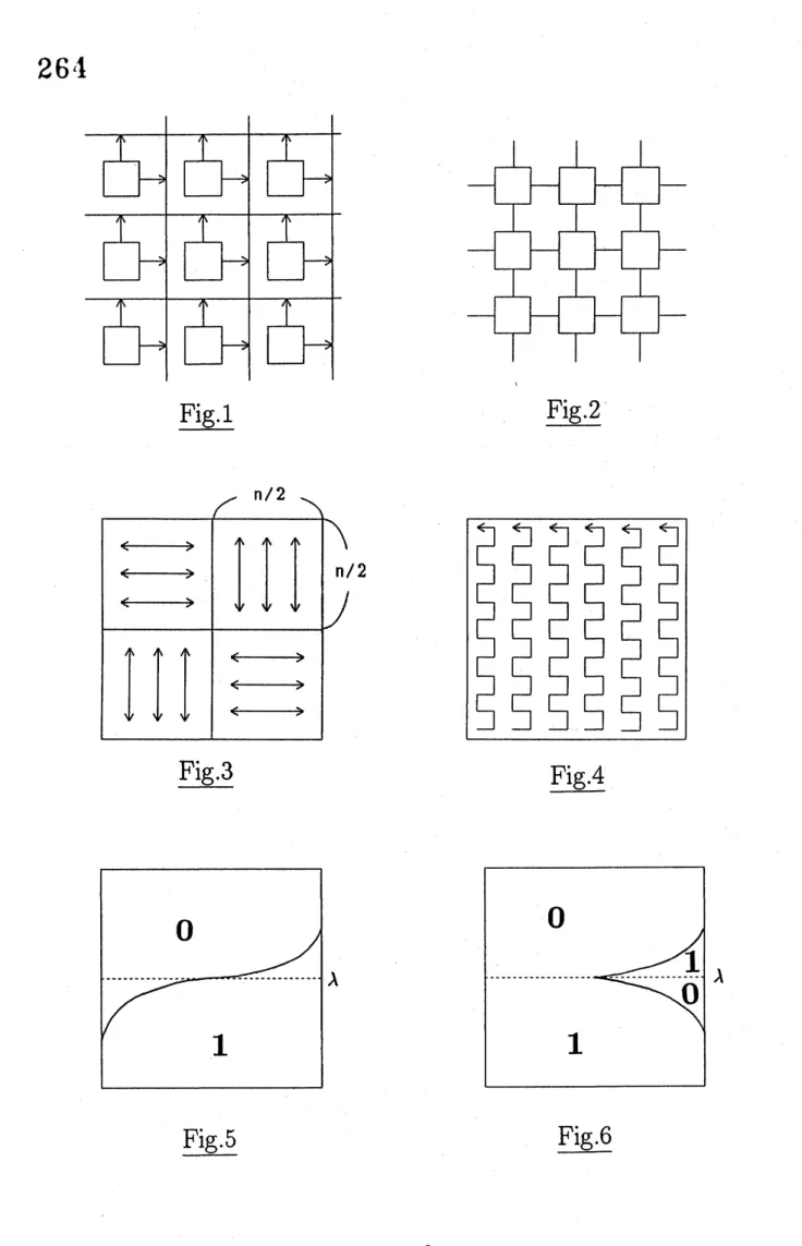
two dimensional paraUel model, caUed the mesh-buscom-$P^{uter}(MC,$ $i_{ig.2)withrowandco1umnbusesInthispaper,weapp1yabenchmarktest’ tothi^{1}}^{MB,Fig.1),byrep1acingthe1oca1.connectionsofthecommonmesh- connectedcompute_{s}}\backslash$’
new model $MB.$by selecting five typicalproblems appearing often in the literature. The result
is alittle surprlslng; it
seems
quite reasonable to claim MB’s superiority ovel $MC$.
Out of thefiveproblems, $MB$ is clearly better than $MC$ for three and is not worse for the rest.
Thefiveproblemsinclude graph connectivity,findingmaximum, semigroupopera.tions,
routing$aItd$sorting. They take $nxn$data($nxn$incidence $mat_{1}\cdot ices$ for graphs)as their inpnts.
Forthefirsttwo problems, $MB$allowsustodevelop logarithmic depth algorithms,whilc $MC$ has
$\circ ve^{I}rMCbutl.5n(l.0nforsomeuseat\cdot ivia1l\circ werbound\circ f\Omega(n)(see[2\iota_{u1subsetsofinstances)isenoughonMB.M^{1}ostsemig\cdot\circ t1I)}^{f\circ rgraphprob1ems).Routingalsoneedst\cdot ivia12ns_{1}teps}$
$o\iota)erations$ are carried out in time $\Theta(n)$ over both MB and $MC$
.
For $several_{1}\cdot easonsme1$)$1i_{ottC^{\backslash }}d$later, sorting is probably the hardest problem for $MB$
.
We nevertheless present, as the lnostsignificant result of this paper, an $O(n)$ randomized algorithm; called the binomial curve $so\iota\cdot t$,
which depends on only row (column)-based sorting.
Note that MB and $MC$ areincomparable in theworst case analysis, namely, it is not
hard to think of triviaJ operations for which either of them needs $\Omega(n)$ steps to simulate the
$o_{atura1pro}n^{ther’ sO(1}l_{1emsinc1udingnoton1ytheabovefive\circ nesbutmanyothers.Itseemshardtofi\tau d}^{steps.H\circ wever,ourmainc1aimappearstobequite1egitimatefornontrivia1a_{l}nd}$
such problemsfor which $MC$ is essentIally better than$MB$ and this$wiU$ be anice talget for the
future study.
Remark 1. Thereis ahuge literatureon themesh-connected computers. Also a$fai_{1}\cdot 1y$
large number of papers discussed mesh-type bus-communication [1] [3] [11] [12]. Howevel$\cdot$
, all
ofthem introduced the bus-communication as an addition to the local connections in order to
avoid the large diameter of mesh-connected computers. To supply with both buses and local
connections may seem an easy and reasonable solution but actually is not: There is a $\backslash vide$
agreement that the degree of integration depends on the number of communicationlines $rathe\iota$
.
than onthenumber of logic gates. If this statement istrue, and ifwe make arough $estin\tau ation$,
to use both buses and local connections needs doubled space for low and $co1_{U1}nnd;_{1CC}tions$
.
It then needs four times as large space as either only buses or only local connectiotls. or $tlle$
maximum number of processors for alimited space becomes one fourth.
Remark 2. Even ifwe do assumethat busesand local connections areboth $avail\backslash .ble$,
the known results do not seem so positive. The most successful one would be the reduction of
time from $n$ (without buses) to $n^{\frac{1}{3}}$
for semigroup operations [12]. For sorting (and proba.bly
for routing) the added buses do not contribute to any reduction of time [11] under the big-O
notation. No logarithmic depth has ever beenreportedfornontrivial problems. Ourachievement
of that $smaU$ depth largely (but not exclusively) depends on our new assumption that $t\backslash voO1^{\cdot}$
mole processors can write data into asingle bus at the same step. It should be noted tha.t
this assumption, although noprevious reports adopted it, is quite natural ifwe realize our bus
systemas abunch of so-called wired-or lines. Our regulation for the simultaneous write is called
BUS: If the written values are $aU$ the same then the value survives. Otherwise, $i.e.$, if $diffel\cdot ent$
valuesarewritten,then the coUision is theonly informationwe know. Note that wedo not need
the simultaneous write for the$O(n)$ algorithms.
Remark$. Both$MB$and$MC$ canbe regardedasthe$paraUel_{1^{\backslash }}andom$accessmachines
(PRAMs) withrestriction: $MB$ can only use $2\sqrt{N}$memory ceUs for $N$ processors but each cell
can be accessed&om $(fixed)\sqrt{N}$processors. (BUS regulation is weaker than ARBITRARY.)
$MC$ can use about $N$ ceUs but each $ceU$ can be accessed from only two processors. (It is anice
propertyfor parffiel models that theycanbe simulated by PRAMs with asimilaror lessamount
of
resources
in thesense
that the models at least do $not$ violate the rule of the most standardmodel. It should be noted that recently developed reconfigurable arrays [13] do not have this
property.)
数理解析研究所講究録 第 754 巻 1991 年 257-266
258
2.
Graph
Connectivity and Finding
Maximum
Algorithms in this section
are
randomized and need the simultaneous write.Theorem 1 [5]. Suppose that each of$n\cross n$ processors initially holds each value of an
$nxn$ incidence matrix of agraph $G$
.
Then we can compute connected components of$G$ overMB ($BU6$ regulation)in $O(\log n)$expected time.
Thus the performance of MB does not differ so much from CRCW-PRAMs for this
particular problem [10]. We conjecture that MB also has (poly)log-depth algorithms for other
graph problems like obtaining a minimum spanningtree. Thisconjecturewouldbestrengthened
by thefollowing result:
Theorem2. MB (BUS regulation) canfind amaximum among$nxn$ data in $O(\log n)$
expected time.
Proof(Sketch). Using the randomized procedure mentioned later, we first try to pick
out a single data, at random, among $n$ ones per each row, using constant steps. It is not
necessary to actuaUy succeed in doing sofor all the rows but is enough to succeed for “many”
rows. Thenwegather those datato the processors at the diagonal position and wecompute the
maximum amongthose (at most n) data in constantsteps using the standard technique. Then
allthe processors know this maximum $M$ through buses and “kill” its owndata if it is less than
$M$
.
Now the number of live data should be reduced, ideally, from $n^{2}$ to some$n$, or a constant
number per row on average. This might be too optimistic but we can certainly expect, with a
good probability, that the largest number of live data on any single row is reduced to a factor
of $\frac{1}{c}$ for some constant $c>1$
.
Nowwerepeat this operation. Again we wish to pick out asingle data for all the rows
orat least for therows on whichalarge number of data remain live. Then the number of those
datashould be reduced to a factor
of}
again and so on.Roughly $Thekeytoolforthisoperationistheprocedure,cat1edPickOne,int\cdot oducedin[5]_{;}speaking,eachprocessoronasinglerowho1dinga1ivedat\overline{a}triesto^{1}raiseaflag$’
with probability $q$ ($= \frac{1}{n}$ initially). If no processors on that row actually raise flags, then they
simply finish that iteration of the procedure’s main loop after executing$q:=2q$
.
Otherwise, if,fortunately, exactly one pro’cessor actuaUy raises a flag, then it is picked out. If two or more
processors raise flags (wecan tellthat fact thanks tothe BUS regulation) then theyfurther try
to pick out exactly one among them using a constant steps (e.g., by trying to raise flags again
with probability, say, $\frac{1}{2}$). $\square$
3.
Routing
In the restof the paperno algorithms assumethe availability of thesimultaneous write. (It does
not seem towork effectively for the restof theproblems.) All the algorithms in this section are
deterministic. Routing is the following problem: Given $nxn$ pairs of (data, destination) $s$, we
are supposed to move $aU$ the data to their destinations. We need asomehow precise definition
for one-step computation, which includes (i) reading the data on both row and column buses,
(ii) executing constantstepsof local computation and(iii) possiblywritingdataintorow $and/or$
columnbuses. It is easy todevelop anelementary algorithm for routing which runs in $2n$ steps.
Our improved result is:
Theorem 3. 1.$5n$ steps areenough for routing over MB.
Proof(Sketch). $nxn$ processors are divided into four $\frac{n}{2}x\frac{n}{2}$ ones. Using the first
$\frac{n}{2}$ steps, we move upper-left $\frac{n}{2}x\frac{n}{2}$ data, $sequen\dot{t}ially$ from left to right, horizontally to their
correct positions with respect to column (see Fig.3) The lower-right $\frac{n}{2}x\frac{n}{2}$ data are also moved
horizontaly and the rest half of data are moved vertically in a similar fashion. Note that a
single processor may hold up to $n$ data at this moment. Using the next $n$ steps, we move all
those data (at the correct positions eitherin row or column) to their final positions. They are
put on the buses not in the order of their current positions as before but in the order of their
destinations.
$\square$In this algorithm, we can reduce the $n$ steps of the second stage into $\frac{n}{2}$ steps if the
input has some regularity. Those regularities include practical ones such as the transposition
and the ls0 rotation.
For this problem, a lower-bound analysis might be more interesting. We have the
following result under the assumption that (i) every data written on a bus must be one ofthe
259
Theorem 4. Suppose that the input data can take the value up to $C$
.
Then if$C>(\alpha n)^{\frac{\alpha}{1-a}}$ for a constant $\alpha(<1)$, thenrouting needs morethan $\alpha n$steps (Proofwill be given
in a future report).
It should be noted that the condition $C>(\alpha n)^{\frac{\alpha}{1-a}}$ only says that the number of bits
for each data is up to $\frac{\alpha}{1-\alpha}\log n$
,
which is quite reasonable, even if we set $\alpha\approx 1$, for a large $n$.
Thus the theorem gives us the lower-bound of roughly $n$ steps. It seems difficult to narrower
the gap between 1.$5n$ and $n$
.
4.
Sorting
Alot of$O(n)$ algorithmsover MC have been developed (e.g., [7] [9]). Their common techniques
include: (i) Recursive divide-and-conquer (typicaUy, dividing the whole $nxn$ into four $\frac{n}{2}x\frac{n}{2}$
bus system is quite undesirable to those methods since the buses cannot be “cut”. Our new
binomial curvesort (BCSORT) depends onlyon row (column)-basedsorting and makes full use
of the randomization.
We first introduce a simpler version of BCSORTtomake thebasic ideaclear. The input
datais givenas an$nxn$array, which wesortinto the snake-like row-major order. To randomize
$a$ row(a column) means to permute the elements on that row (column) at random. We can do
sobygenerating randomnumbers, onefor eachelement, and then sortingthe elements by those
random numbers.
Algorithm BCSORT-I:
Step 1. Randomize allrows.
Step 2. Randomize all columns.
Step 3. Sort all columns from top to bottom.
Step 4. Sort all odd-numbered rows from left toright and all even-numbered rows from right
toleft. (That is caJled shearingin [8]). Test if the sorting is completed, and stop if it is.
Step 5. Sort all columns from top tobottom.
Step 6. Randomize $aU$rows. Go to Step 3.
To execute each of Step 1 to Step 6, we apparently need $\Omega(n)$ steps for both MB and
MC. For MB, a method called “counting sort” seems to be convenient. Each element is placed
on the bus in a regular order while the other elements know their positions by counting the
number ofsmaller elements. To achieve$O(n)$ total running time, therefore,we have to keep the
number of iterations from Step 3 to Step 6 within $O(1)$
.
We shaJl take alook at the behavior of the algorithm whentheinput consistsof only$0’ s$
and 1$s$ (see Lemma 1 forourversion of the$zero/one$-principle.). Wealso assume, for simplicity,
that the number of l’s is exactly $\lambda n$, for some integer $\lambda\leq n$
.
Steps 1 and 2 deliver all l’s atrandom on the $nxn$ plane (actually Step 2 is not necessary). Step 3 moves all l’s towards
the bottom. Suppose, hypothetically, that we sort all rows to the right after that. The result
would look like Fig.5. One can see that the curve becomes close to the binomial distribution
$b(k, n, \})$, i.e., (the number of columns including $k$ l’s )$/n$ should be nearly equal to $b(k, n, \frac{\lambda}{n})$
.
Again, suppose hypothetically that we can change the direction of rows (from left-to-right to
right-to-left)at the$\lambda’ th$ row asin Fig.6. It isawell-known fact that the twocurves onboth sides
ofthe border (the $\lambda’ th$ row) are nearly symmetric unless $\lambda$ is close to zero. This implies that
ifwe sort columns again, then both the l’s misplaced above the border and the $0’ s$ under the
border would be “neutralized” almost completely. In reality, however, we cannot know where
the border is, and for a general input, such a border does not exist. Fortunately, Step 4 has
almost the same effect as changing the direction at the $\lambda’ th$ row, which will be shown in the
next section.
Thus, the configuration after Step 5 should look like Fig.6, where most of
wrongly-placed $0’ s$ and l’s stay very close to the border. If these $0’ s$ and l’s stay only on either the
A’th row
or
the$(\lambda+1)st$ row (i.e.,$0s$ on A’th and l’s on $(\lambda+1)st$), then one can see that theywill definitely move to the right place in the next iteration. Otherwise, Step 6 plays its role.
260
Such apileis dangerous since (ifStep 6 ismissing) its height may decrease only by halfduring
asingle iteration. By Step 6, however,these piles are demolished evenly and the probability of
encountering such piles again in the next iteration should be decreased greatly.
This observation dependson akey assumptionthat thebinomialcurvein Fig.6 or Fig.7
is nearly symmetric. However, it is also well known that it is not the case if$\lambda$ is smdl. Then
we should encounter, not accidentally, alarge number of the high pilesmentioned above. It is
not clear any longer if Step 6 can manage the situation only byitself. Here is our algorithm in
a complete form:
Algorithm BCSORT-II:
Step 1- Step 5. Exactly thesame as thesimplified version above.
Step 6. Partitiontherowsinto “layers”. Borders between thelayersareat 4th row, 8th, 16th,
32th, ...,$2^{:}th,$
$\ldots$ from both the top and the bottom rows (see Fig. 8).
Step 7. Randomize allrows.
Step 8. Randomize $aU$ columns within the layers (i.e., any element never goes outside the
borders of its own layer).
Step 9. Shear the rows as in Step 4 andsort all columns again withinthe layers.
Step 10. Sort allrows from left to right (not shearing).
Step 11. See Fig.9. At each row $i$, in the lower halfplane,i.e., $(1 \leq i\leq\frac{n}{2})$, the rightmost $t(i)$
elements (seebelowfor $t(i)$ and the next $s(i)$), denoted by$A$ in the figure, are exchanged
with the same number
of
elements, $B$, beginning with the $s(i)th$ column from the right.We do the samefor the upper half plain but the left most portion is shifted to the right.
Step 12. Repeat Step 3-Step 11 anotherthree times (fourintotal). At the seconditeration,
layering in Step 6 is a little different. The borders set at 5th, 10th, 20th, 40th,
.
..,$(2^{i}+ \frac{1}{4}2^{i})th,$
$\ldots$, i.e., the borders are “shifted” one fourth to the center. In the third
iteration, the borders are shifted two fourths, they are shifted three fourths in the final
iteration.
Step 13- Step 15. Thesame as Step 3- Step 5.
Step 16. Randomize $aU$ rows. Go to Step 13.
$s(i)$ in Step 11is determined as follows:
$s(0)=0$,
$s(i)=s(i-1)+t(i-1)n$
for $i\geq 1$.
Thevalues of$t(i)$ will be defined precisely in the proof of Lemma 2. Roughly speaking, we first
determine its values at the borders of the layers, $t(b_{1}=4),$ $t(b_{2}),$ $t(b_{3})$, and so on. $t(b_{1})$ and
$t(b_{2})$ are given explicitly. Starting from $j=3,$ $t(b_{j})$ is given as $\beta t(b_{j-1})$ for a constant $\beta<1$
.
For rows between the borders, it is given as $t(b_{j}+k)=t(b_{j})\alpha^{k}$ for a constant $\alpha<1$
.
$\alpha$ and $\beta$,given alsoin the proof,
are
fairly $smaU$, and it is guaranteed that $\sum t(i)<1$ for any large $n$.
As mentioned before, we cannot expect a desirable symmetry of the binomial curve
when $\lambda$ is very small, e.g., when
ft
(the ratio of l’s) is $O( \frac{1}{n})$.
Intuitively, we can change thisratioup to some $\frac{1}{4}$ bythe layering and the following operations within eachlayer in Steps 6- 10
.
For the sake of the proof, we want this ratio to be between 0.25 and 0.5. That is the reasonfor Steps 3- 11 to be repeated four times. (It is interesting to see that in Step 8, we “de-sort”
columns that are once sorted.)
In Step 12,we movethe right-endportions of each row,sothat they will neveroverlap
with the
same
portionson the otherrows. The piles of wrongly-placed l’s were collectedtothoseright-end portions by the preceding step. One can see that the piles are thus demolished in a
deterministic fashion rather than in aprobabilistic onein Step 6 of the old simplified version.
The crucial point is tomake the size of those portions large enough toinclude all possible piles,
with, at the
same
time,keeping the total length of the portions within $n$ (the length of a singlerow). As one can seelater, the layering plays akey role to this end. We should not forget that
there is anotherreasonfor the symmetry tobeundermined. Itis “byaccident“. The iteration of
Steps 13-16is introduced tomanagethis indispensableperturbationfor$p^{\Gamma}gol\cdot$
.
Remark 4. BCSORT-I steps within $O$($n$log log$n$) steps with ahigh $p_{1}\cdot obability[4]$
.
[9] presents another $O(n\log\log n)$ deterministic algorithm over MC but based on only row
(column)-basedsorting, which $MB$ cansimulate. We haveaconjecture that BCSORT,Iis much
261
Remark 5. We carried out a simulation for BCSORT-I and its slight modification
BCSORT-III. In the latter,we have Step 5.5 afterStep 5 in which, aftersorting all rows to the
right, the right (left) most elements are shifted to the left (right) as in Step 11. However, we
onlyshift afixed number$(\sqrt{n})$ of elements and thereforetheyoverlap with theircounterpartsof
$eVerBCS^{y}of_{T- I(B\dot{C}SORTIII)ated}^{\overline{n}rowsInTab_{\vee}1e1,T_{j}(T_{3})denotestheaveragenumberofiterations\circ fStep3- 6b_{1}ef_{01}\cdot e}stops.Thenumberoftrialsisatleast50.Inputdatawasgene$
.
at random.
Now we will show our main theorem in this paper.
Theorem 5. BCSORT-II stops at the third iteration of Steps 13-16 with probability
$1-\sqrt{\log n}^{c}$ for some constant $C$:
Twolemmas will be given to justify this theorem.
Lemma 1. Suppose that BCSORT-II sorts any (single) input dataconsisting of only
$0’ s$ and l’s,after executing $k$ “Steps” with probability at least $1-p$
.
Then it sorts any (single)input ofintegers after the same execution sequence of Steps with probability at least $1-n^{2}p$
.
Proof(Sketch). Without loss of generality, we can assume that the general input is
a permutation of $($1,2,
.:.,$n^{2})$
.
The algorithm is oblivious, i.e., its control sequence does notdepend on the values ofinput dataoron the sequence of generated random numbers. Suppose
that the algorithm generates a sequence, $T$, of random numbers. If we fix this sequence, the
algorithm can be regarded as adeterministic one.
Now suppose that the input sequence, $(a_{1}, \ldots,a_{n^{2}})$, is changed to $(b_{1}, \ldots,b_{n^{2}})$ under
the sequence $T$ after the execution of$k$ Steps. If $(b_{1}, \ldots,b_{n^{2}})$ is not sorted, then we can find
the least integer $b_{x+1}$ suchthat $b_{x}>b_{x+1}$
.
(We say that the algorithm does not sort the input$(a_{1}, \ldots,a_{n^{2}})$ at $b_{x+1}$
.
) Now we consider an input sequence $(f_{b.+1}(a_{1}), \ldots, f_{b_{x+1}}(a_{n^{2}}))$ ofonly $O’ s$ and l’s where$f_{b}(a)=\{\begin{array}{l}0ifa\leq b1otherwise-\end{array}$
Under thesame sequence$T$ ofrandom numbers, this input should be turned to
$(f_{b.+1}(b_{1}), \ldots, f_{b_{x+1}}(b_{n^{2}}))$,
exactly as the original $zero/one$-principle [6] claims. Clearly, this sequence is not sortedeither.
Now consider all possible sequences of random numbers of proper length for $k$ Steps.
The discussion above leads us to the conclusion that ifthe algorithm does not sort a (general)
$in(f_{b}^{p_{x}u_{+}t_{1}}t_{a_{1}^{1}),,f_{b_{x+1}^{2}}^{n}(a))withprobabi1ityat1eastqeither.Asaresu1t}^{a,..\cdot.\cdot.’ a)atb_{n^{x+1}}withinkStepswithprobabi1ityq,thenitdoes}$ not sortabinary input
$P_{f}$($(a_{1},$ $\ldots,a_{n^{2}})$ is sorted within $k$ Steps)
$\geq 1-\sum_{b=1}^{n^{2}}P_{f}$($(a_{1},$ $\ldots,a_{n^{2}})$ is not sorted at b)
$\geq 1-\sum_{b=1}^{n^{2}}P_{f}$($(f_{b}(a_{1}),$$\ldots,f_{b}(a_{n^{2}}))$ is not sorted)
Then, the lemma follows since the assumption says that $P,$($(f_{b}(a_{1}),$$\ldots,f_{b}(a_{n^{2}}))$ is not
$sorted_{\square }$)
is at most $p$
.
Lemma 2. BCSORT-II stops for any binary input at the third iteration ofSteps 13-16
with probability $1-2\sqrt{n\log n}^{c}$ for
some
constant $c$.
Proof (Sketch). As before, the probability that asingle column contains $k$ l’s is
de-noted by$b(k,n, \frac{\lambda}{n})$
.
Sincewediscuss asymptotic behaviors,wecan
usethenormal approximationgiven by
$\phi(x)=\frac{1}{\sqrt{2\pi}}e^{-\frac{1}{2}x^{2}}$
for $b( \lambda+x\sqrt{q},n, \frac{\lambda}{n})\sqrt{q}$where $q=(1- \frac{\lambda}{n})$
.
Now suppose that we
are
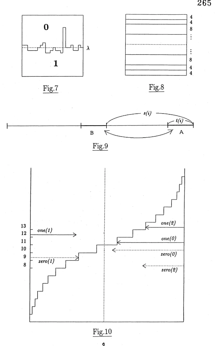
done with Step 3. Ifwe hypothetically sort all the rows to262
${\rm Re} c$all that in Step 4, the direction of sorting is changed at every row. Look at, for example,
the 10th row. If this
row
is sorted to the right, then l’s take the place denoted by one(0) inthe figure. The 9th row should be sorted to the left and the $0’ s$ should stay where denoted by
zero(0), and so on.
Then $aU$ columns are sorted in Step 5. It is convenient for us to consider that by this
sorting$t\acute{h}e$
l’sdenoted by
one
(0)isexchanged with$0s$denoted byzero(0),$one(2)$ withzero(2),..., on the right side of the plane and one$(l)$ with zero(1), $\ldots$, on the other side. We can use
a numerical table for suchsmall $\lambda$ and can verify the followingproperties : (i) zero(i)is larger
thanone(i) where $i$is close to$0$
.
Thereason
is that the largest stair of Fig.10that correspondsto $b( \lambda, n, \frac{\lambda}{n})$ does not exist at theexact center but is shifted a little to the right. $b( \lambda-i,n, \frac{\lambda}{n})$
is larger than $b( \lambda+i, n, \frac{\lambda}{n})$ at the beginning but this relation soon overturns as $i$ grows. (ii)
Hence, at
some
point, one(i) becomes larger than zero(i). This tendency becomes more andmore extreme
as
$i$is getting close to $\lambda$.
Therefore, after the column sorting, the configurationcan be shown as in Fig.11. Recall that the average is $\lambda(=10)$
.
Below the average we findwrongly-placed $0’ s$onlyon the 10th row,wefind wrongly-placed l’s onbothleft and rightends,
which can become relatively tall piles. It should be noted that this observation also holds for
larger $\lambda$
.
Now we are going tothe next important step, Step 8. Recall that we repeat Steps
3-$borderbetween0’ sandl’ sfitthethirdlayer(beginningwiththe9throwandendingwith16thllfourtimeswithslightlychangingthelayering.Suppose,aain,that\lambda=l0.Thenthe(final\{$
in the firstiteration. That layercan beregardedasincluding about $\frac{1}{4}$ l’s and $\frac{3}{4}0s$
.
After Steps9and 10,wewill againencounter,asin Fig.11, thewrongly-placed $0s$on the 10th row andpiles
of wrongly-placed l’s at both left and right ends. Thistime, however,oneshouldnotice agreat
difference; the ratio of l’s is changed from very small $\frac{10}{n}$
to}.
We can show that this new ratiois large enough to claim that these l’s piles only appear at the “far end” of the row as follows:
In this specific example, we can calculate explicitly the values of $b(0,8, \frac{1}{4}),$ $b(1,8, \frac{1}{4})$,
...,
$b(8,8, \frac{1}{4})$,
which shows that (i) $b(2,8, \frac{1}{4})$ is the largest, (ii) $b(0,8, \})$ and $b(1,8, \})$ are veryclose to$b$(4, 8,
})
and$b(3,8, \})$,respectivelyand(iii)$b(5,8, \})$,$b(6,8, \frac{1}{4})$ and so on are very small.
In otherwords,the l’s piles
can
onlyappearaccording to$b$(5,8,}), .
..,$b(8,8, \})$.
It is not hardto show this in general, i.e., weonly have to consider the l’s piles according to $b(2wp+i, w,p)$
for $i\geq 0$, where $w$ is the width of thelayer and$p$ is theratio of l’s inside that layer. Since we can assume $\frac{1}{4}\leq p\leq\frac{1}{2},$ $b(2wp,w,p)$ becomes maximum (the worst case for us) at$p= \frac{1}{4}$
Now weare readytodetermine the value of$t(i)$ usedin Step 11. When$w(=the$width
of thelayer)is8,$b(5,8, \frac{1}{4})+\ldots+b(8,8, \frac{1}{4})<0.04$, which is enough for$t(8)$
.
Similarlywetake0.06for $t(0)$ and $t(4)$
.
$b(2wp+i,w,p)$ decreases sharply as $i$ increases and therefore we can choose,e.g., $\frac{1}{4}$ for factor $\alpha$
.
Using the normal approximation one can also verify that $b(4wp, 2w,p)$ ismuch smaller than $b(2wp, w,p)$
.
Therefore we can choose, e.g., $\frac{1}{4}$ again for $\beta$.
Thus, by theshifting operation in Step 11, all of the wrongly placed l’s are completely distributed so that
any two ofthem neveroccupy the same column. That means all the wrongly placed $0’ s$ and l’s
are gathered toonly twoconsecutive rowsafter Step 13 and the algorithm must stop at Step 14
with probability one!
Ofcourse that is too optimistic since the discussion so far assumes that the
distribu-tion of $0’ s$ and l’s completely follows the theoretical distribution. Consider, for example, the
probability,$p(h)$, that arow contains $(\lambda+h\sqrt{q})$ l’s or more. The normal approximation gives
us, for example,nearly 0.16as$p(1)$
.
It should be noted that the actualnumber, say $\#(h)$, ofsuchrows
can
change again following the binomial distribution. Let $m$ be the number ofcolumns,which we wish todistinguish with $n=the$number ofrows. Then the random perturbation to
$\#(h)$ should follow the distribution
curve
whose expected value is$p(h)\cdot m$ and whose standarddeviationis roughly $\sqrt{p(h)m}$if$p(h)\ll 1$
.
$p(h)= \int_{-}^{h_{\infty}}\phi(y)dy\approx\frac{1}{h}\phi(h)$
iswell known
as
agood approximation. Onecan
easilyverify that$p( 2\sqrt{ogm})=1-\frac{l}{2\sqrt{\pi\log m}\cdot m^{2}}$.
It means that $\#(h)$
can
change from its expected value $mp(h)$ by at most263
ifwe guaranteeour desired probability $1- \frac{l}{2\sqrt{\pi\log m}\cdot m^{2}}$
.
Note that the number of columns containing exactly$(\lambda+h\sqrt{q})$ l’s is
$m\cdot\phi(h)/\sqrt{\lambda q}$
.
(2)It follows that the random perturbation given by (1) can create the “pile” ofwrong l’s whose
height can be up to
(1)$\div(2)=2\sqrt{\frac{\lambda q\log m}{m}}\cdot\frac{1}{\sqrt{h\phi(h)}}$
Since this pile is created with probability $p(h)$
,
its average height should be(3) because $m>\lambda q$ and $2\sqrt{\phi(h)}/h\sqrt{h}\leq 1$ for $h>1$
.
Now for the seconditeration of Step13-16wecan repeat the above discussion by setting
$\lambda=\sqrt{ogm}$
.
At the thirditeration, $\lambda$is again reduced to $(\log m)^{0.75}/m^{0.s}$ byformula(3), whichis enough forus since we
can
conclude: The probability that the wrong “piles” of height one ormore appear is at most
$\frac{(\log m.)^{0.375}}{m^{025}}\cdot\frac{1}{\sqrt{2\pi}}e^{-\frac{1}{2}\frac{m^{0.5}}{(1\circ\iota n)^{O.75}}}$,
which becomes infinitely small for large$m$
.
Thus there are two undesirable phenomena, the antisymmetry ofthe binomial curve
when $\lambda$ is small and the difference from the theoretical curve caused at random. We have
discussed those two independently, which should be combined in a formal proof. One can see,
however, that the first phenomenon is important when $\lambda$is small and the second when $\lambda$islarge.
Furthermore, by slightly more detailed analysis, we
can
show each is negligible where we haveto consider the other. The detailed proof is left to the full paper. $\square$
References
[1] A.Aggarwal, “Optimal Bounds for Finding Maximum onArrayof Processors with$k$Global
Buses”,IEEE Thans. Comput., C-35, 1, pp.62-64, 1986.
[2] M. Atallah and S. Kosaraju, “Graph Problemson a Mesh-Connected ProcessorArray”, J.
ACM, 31, 3, pp.649-667, 1984.
[3] S. H.Bokhari, “FindingMaximumonanArrayProcessor with aGlobalBus”,IEEE Trans.
Comput., C-33, 2, pp.133-139, 1984.
[4] H. Imai, personal communication, 1991.
[5] K. Iwama and Y. Kambayashi, “An $O(\log n)$ parallel connectivity algorithm on the mesh
ofbuses”, Proc. 11th IFIP World Computer Congress, pp.305-310, 1989.
[6] D. Knuth, “The art ofcomputerprogramming”,Addison-Wesiey, 1973.
[7] H. Lang and M Schimmler and H. Schmeck and H. Schroder, “Systolic sorting on a
mesh-connected network”,IEEE Trans. Comp., C-34, pp.652-658, 1985.
[8] Scherson and Sen and Shamir, “Shear sort; A true two dimensional sorting technique for
VLSI networks“, Technical Report, University ofCalifornia, Santa Barbara, 1985.
[9] C. Schnorr andA. Shamir, “Anoptimalsorting algorithms for mesh connected computers”,
18th ACM Symposium on Theory ofComputing, pp.255-263, 1986.
[10] Y. Shiloah and U. Vishkin, “An $O(\log n)$ parallel connectivity algorithm”, J. Algr., 3,
pp-57-67, 1982.
[11] Q. F. Stout, “Mesh-connectedComputers with Broadcasting”, IEEE Trans. Comput., C-32,
9, pp.826-830, 1983.
[12] Q. Stout, “Meshes with multiple buses”, Proc. Proc. 27th IEEE Symp. on Foundations of
Computer Science, pp.264-273, 1986.
[13] B. F. Wang, G. H. Chen and F. C. Lin, “Constant Time Sortingon a ProcessorArray with