A Hybrid Method for Solving the Nonlinear Least Squares Problem with Linear Inequality Constraints

(1)

Society of Japan

Vol. 38, No. 1, March 1995

A HYBRID METHOD FOR SOLVING THE NONLINEAR LEAST SQUARES PROBLEM WITH LINEAR INEQUALITY CONSTRAINTS

Nobuko Sagara Masao Fukushima

Aichi University Nam Institute of Science and Ttchnology

(Received January 6, 1993; Final October 12, 1994)

Abstract This paper presents a new method with trust region technique for solving the nonlinear least squares problem with linear inequality constraints. The method proposed in this paper stems from the one presented in a recent paper by the authors. The method successively constructs trust region constraints, which are ellipsoids centered at the iterative points, in such a way that they lie in the relative interior of the feasible region. Thus the method belongs to the class of interior point met.hods, and hence we may expect that the generated sequence approaches a solution smoothly without the combinatorial complications inherent to traditional active set methods. 'Ye establish a convergence t.heorem for the proposed method and show its practical efficiency by numerical experimenl.s.

1. Introduction

In [16]' we have proposed an algorithm for solving nonlinear least squares problems with simple bounds. The purpose of this paper is to generalize the results of [16] to problems with linear constraints. Although the constrained linear least squares problem has extensively been studied [1, 2, 3, 6, 8, 12, 17], less attention has been paid on the constrained nonlinear least squares problem. Holt and Fletcher [9] consider the nonlinear least squares problem with simple bounds and monotonicity constraints on the variables. Wright and Holt [20] extend the results of [9] to general linearly constrained problems by utilizing the structure of the sum of squares objective function. For the problem with nonlinear equality constraints, Knoth [11] gives a generalized Gauss-Newton method with stepsize strategy based on an exact penalty function. Mahdavi-Amiri and Bartels [13] consider an exact penalty method to solve the problem with nonlinear constraints and use quasi-Newton updates that take into account the structure of nonlinear least squares Hessians. Schittkowski [18] considers SQP methods to solve nonlinearly constrained least squares problems.

In this paper, we consider the following nonlinear least squares problem with linear inequality constraints:

minimize

!

t

F;(x? 2 ;=1

(1.1 ) subject to AT x :::; b, x ~ 0,

where x E Rn, bERm, A E Rnxm and Fi : ~ --. R, i = 1,···, i, are continuously differen-tiable. We define the functions F : Rn --+ Ri and

f :

Rn --+ R by F(x) = (F1(x),···, Ft(x)f

(2)

56 N. Sagara & M. Fukushima

Using slack variables yE Rm, we may rewrite problem (1.1) as

minimize

f(x)

subject to AT x

+

y = b,

x;:::

0,

y;:::

o.

(1.2)

The method proposed in this paper stems from the one presented in [16]. Specifically, the method constructs trust region constraints, which are ellipsoids centered at the iterative points, in such a way that they lie in the relative interior {(x, y)

I

AT X

+

y = 0, x > 0, y > o}

of the feasible region of (1.2). Thus the method belongs to the class of interior point methods. However, since solutions of the problem are usually on the boundary of the feasible region, the trust region ellipsoids may become extremely thin, which causes numerical instability. To avoid this difficulty, we incorporate an active set strategy into the method. With such a modification, we may still expect that the method retains the advantage of the interior point method, as observed in [16] for the case of problems with simple bound constraints on the variables.

The paper is organized as follows. Section 2 presents motivation and description of the algorithm. In Section 3, we establish a global convergence theorem. Finally, in Section 4, we report some computational results with the proposed algorithm compared with the successive quadratic programming method.

2. Algorithm

First, we describe a basic idea of the algorithm. Suppose that (x, y) is a relative interior point of the feasible region of (1.2), i.e., AT x

+ y

= b, x

>

0, y

>

O. Let p and q denote the vectors which determine the next points (x+, y+) from the current point (x, y), that is x+

=

X

+

p and y+

=

Y

+

q. We consider the following Gauss-Newton type subproblem with

an additional trust region constraint:

minimizep,q

211

1 F(x)

+

V'F(x)Tp

112

subject to ATp+q

=

0,

11

D(x)p

112 +IID(y)qI12 ::;

~2,

where D(x) = diag(l/xi), D(y) = diag(I/Yi) and ~ is a constant such that 0

<

~

<

l.

This problem can be rewritten as

minimize p,q subject to 1 g(x)Tp +

2

PTH (x)p ATp+ q = 0, IID(x)pIl2

+ IID(y)qI12 ::;

~2, (2.1)

where H(x)

=

V' F(x)V' F(xf and g(x)

=

V' F(x)F(x). Note that if (p, q) satisfies AT p+q =

0, then (x+,y+)

=

(x,y)

+

(p,q) also satisfies ATx+

+

y+

=

b. Also, if (p,q) satisfies

IID(x)pI12 + IID(y)qI12 ::;

~2, then x+ and y+ remain in the relative interior of the feasible region, i.e., x+

>

0 and y+

>

o.

In fact, if xt ::; 0 for some k, then it follows that

(3)

This implies that

IID{x)pI12

+

IID{y)qIl2

=

~

(::)

2

+

~

(::)

2

>

(Pk)2 2: 1, ,Xk

contradicting IID(x)pI12

+

IID(y)qI12 :::; 6.2

<

L Hence, x+

>

0 must hold, In a similar manner, we can show y+

>

O. To guarantee convergence of the method, we control the size 6, of the trust region according to the ratio of the actual and predicted reductions caused by the step (p, q) chosen to determine the next iterate.

The trust region constraint IID{x)pI12

+

IID(y)qI12 :::; 6,2 in (2.1) represents an ellipsoid, which is centered at the current point (x, y) and strictly contained in the nonnegative orthant

{(x, y)

I

x 2:

0,

y 2:

O}.

However, when the current point is close to the boundary of the nonnegative orthant, the trust region ellipsoid becomes thin and solution of (2.1) suffers from numerical instability. To overcome this dHficulty, we modify (2.1) using the idea of active set strategy [5] in constrained optimization.

For the current point (x, y), we define the sets of indices

I={ilxi2:

E

d,

J:={jIYi2:

E1}, (2.2)

where El is a sufficiently small positive constant. We also denote

1

= {I, 2" .. ,n} - I and

J

=

{I, 2, .. " m} - J. According to the above definition, we partition vectors and matrices as

() _[9I(X) ]

9 X = .fJI(x) ,

By adding the extra constraints PJ

=

0 and 'lJ

=

0 to (2.1), we get the following problem:

minimizepI •v 9I(xf PI

+

~pf

HII(x)PI subject to A;JPI

=

0, AfJPI

+

qJ

=

0, IIDI(X)PIII2

+

IIDJ(y)qJI12 :::; 6,2, (2.3-a) (2.3-b) (2.3-c) (2.3-d) where DI(X) and DJ(y) are the diagonal submatrices of D(x) and D(y) with elements l/xi,

i E I, and l/Yi' j E J, respectively. Note tha.t by the definition (2.2) of I and J, the following inequalities are always satisfied:

Thus any (Ph qJ) satisfying

11 PI 112

+

11 qJ 112:::; E~6,2

also satisfies the inequality d). This fact implies that the ellipsoid determined by (2.3-d) contains the sphere with radius E1d. So the ellipsoid never becomes thin as long as the

(4)

value of ~ does not approach zero. (The latter property will be shown to hold in the proof of Theorem 3.1.)

Now, as qJ = -AJJpr by (2.3-c), from (2.3-d) we have

P; Dr(x)2PI

+

qr

DJ(y)2 qJ

=

P; (DI(X)2

+

AIJDAy)2 A;J) PI ~ ~2. Thus, we can rewrite (2.3) as

where E( x) is defined by

minimizep1 gr(xf Pr

+

~P;

HII(X)pr

subject to AJ]pr = 0, pr E(x)Pr ~ ~2,

E(x)

=

Dr(x)2

+

AIJDJ(y)2 A;J

=

Dr(x)2

+

AIJDAb - AT X)2 ArJ'

(2.4)

(2.5) where the last equation follows from the fact that (x, y) is feasible to (1.2). In the remainder of the paper, we suppose that the following two conditions are always satisfied:

rankAr]

=

111,

ZT HII(X)Z is positive definite,

(2.6) (2.7) where Z is a

I

I x(III - 111)

matrix whose columns span the null space of AJ]" Note that (2.6) is satisfied when (1.2) enjoys the primal nondegeneracy condition, provided that El is

chosen sufficiently small.

Let a solution pj of (2.4) be obtained. Suppose that

Ilpill

2

E2 is satisfied, where E2

is a predetermined positive number significantly smaller than El. If the value I(x

+

p*) is

sufficiently smaller than 1(3.~), then we accept p. to determine the next point. Otherwise, we halve ~ and solve subproblem (2.4) again. More precisely, let 0

<

11-

<

TJ

<

1, 'Y

>

1 and

o

<

~ma.,

<

1 be given constants. Compute the ratio

_ I(x

+

p*) - I(x)

P = 1f;(x,p*) , (2.8)

where 1jJ(x,p) = g(xfp

+

~pT H(x)p. If p

<

11-, then put x+ := x and ~ + := ~~; if

11- ~ P

<

TJ, then put x+ := x

+

p* and ~ + := ~; if P

2

TJ, then put x+ := x

+

p* and ~+ := minCt~, ~ma.,). When x is updated, i.e., x+ = x

+

p*, we compute y+ := y

+

q*

2

0, where qj = -AIJT pi and

qj-

= o.

With the next iterative point (x+, y+), we update the index sets I and J by (2.2). As a result, we have problem (2.4) corresponding to the new index sets I and J. In this manner, we repeatedly solve subproblems (2.4) while updating the index sets I and J as long as

Ilpi

11

2

E2 holds.

On the other hand, if

Ilpill

<

102 is satisfied, then we may regard the current point x as

an approximate optimal solution of the problem minimize

I (

x )

subject to AT x + y

=

b,

Xy

=

O,Y]

=

O.

(2.9)

This can be verified as follows. When pi is small, so is qj = -A;JPi by (2.3-c). Since the ellipsoid determined by (2.3-d) contains the sphere with radius E1~ as noted earlier, we may

(5)

think that the constraint (2.3-d) is inactive at the solution (pj, qj) of problem (2.3), when ~ is not too small. (Recall that E2 was chosen significantly smaller than Ed Therefore, (pj, qj) satisfies the following optimality condition for problem (2.3) with constraint (2.3-d) being ignored:

gI(X)

+

HII(X)PI

+

AIJ;\:J+ AIJAJ 0, (2.1O-a)

AJ 0, (2.10-b)

A;JPI 0, (2.10-c)

AiJPI

+

qJ 0, (2.10-d)

where A is the Lagrange multiplier vector and (AJ, AJ) is the partition of A corresponding to the index set J defined by (2.2). If (pj,qj) satisfying (2.10) is sufficiently small, then the point x may be considered to approximately satisfy

(2.11) which is actually the optimality condition for problem (2.9).

So in the case where 11

pi

11

<

E2 is satisfied, we have to further examine optimality of

the point x for the original problem (1.2). Namely, we compute Lagrange multipliers AJ by solving the equation

A;JArJAY = -A;JgI(X)

and check if Ay satisfies the inequalities

gy(X)

+

AIJAy:::· -E3e,

Ay::: -E3e,

(2.12)

(2.13) (2.14) where E3 is a sufficiently small positive constant and e is a vector of appropriate dimension

whose components are all unity. Note that, by assumption (2.6), equation (2.12) ha.., the unique solution AT' If (2.13) and (2.14) hold, then we terminate the iteration, since the definition of I and J implies that (x, y) satisfies approximate optimality conditions for problem (1.1), which depend on 101,102 and E3.

To see this, note that the Kuhn-Tucker conditions for problem (1.2) are given by

which imply g(X)

+

AA:::: 0, x:::: 0, xT(g(x)

+

AA)

=

0, A :::: 0, y:::: 0,

)7

y = 0, 9Jo(X)

+

_AloJoAJo= 0, f/[o(x)

+

_{AloJoAJo ::::}0, AJo = 0, AJ_{o ::::}0, Xlo :::: 0, X10

=

0, YJo :::: 0, YJ_o= 0, (2.15-a) (2.15-b) (2.15-c) (2.15-d) for some partitions (Io,lo) and (Jo,

J

o) of {1, 2"", n} and {1, 2"", m}, respectively. In

view of the definition (2.2) of I and J, we see that (2.13) and (2.14) are relaxations of conditions (2.15-b) and (2.15-d), respectively. Moreover, (2.15-a) and (2.15-c) correspond to (2.10-a) and (2.10-b), which approximately represent condition (2.11) when (pj, qj) is

(6)

sufficiently small. In the following, conditions (2.13) and (2.14) will simply be referred to as E-optimality conditions for problem (1.1), with E

=

(El,E2,E3)'

When any of the conditions (2.13) and (2.14) is violated, we try to improve the current solution by solving subproblem (2.4), in which the index set I or J is modified. Specifically, if (2.13) is violated, we let the currently active variable Xi' be inactive, where index i* is determined by

i* := arg max{

I

(gy(x)

+ AIJAY}i

I

(gy(x)

+

AIJAY}i

<

-E3, i E

I},

namely, we let

1:= 1-

{i*},

1:= I U

{i*}.

Similarly, if (2.14) is violated, we let the currently active variable Yj* be inactive, where

index j* is determined by

j* ::= arg max {

IAjl1 Aj

<

-E3, j E

J},

namely, we let

J

:=

J -

{j*}, J:= J U {j*}.

By means of this manipulation, we may expect to improve the current solution by solving subproblem (2.4) with the revised active sets. In fact, let the condition (2.13) be violated and the index set I be augmented by i*. To be precise, we denote j

=

I U {i*}. Then, since

IIpill

is small, the current solution X approximately satisfies (2.11), i.e.,

(2.16) and

i*

is such that

(2.17) Now suppose that, on the next iteration, the solution x fails to be improved by solving (2.4) with the revised active set

i.

Then we must have

IIpill

~ 0 again for the current solution x,

so that x approximately satisfies

for some

'\y,

i.e., we have approximately

gI(X)

+ AiJ,\Y

gi* (x) + AioJ,\y 0,

o.

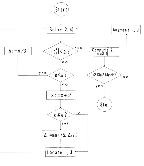
(2.18) (2.19) However, since AIJ has full column rank, (2.16) and (2.18) imply that the vector '\Y is approximately equal to Ay, which contradicts (2.17) and (2.19). So when (2.13) is violated, an improvement will be obtained on the next iteration. The case where the condition (2.14) is violated can be argued similarly.

We are now ready to state an algorithm for finding an E-optimal solution of (1.1). An outline of the algorithm is shown in Figure 1.

(7)

r - - - - . - - - I L - - - _ - - - - r -_ _ 1 - - - 1

A

u gme n

t

I

~

*

~yes

11

Pr

11

<

£2

l

_/

/>---1

Comp

_by(2.12)

u

t

e

1J

/J. : =/J./2 ]

no

yes

(2.13),(2.14 )hold?

_no

yes

L - -_ _ _ _

~

_ _ I

Up d

ate

I,

J

r'~---'

(8)

Algorithm

Initialize: Choose sufficiently small positive constants Ei, i = 1,2,3, and parameters

/-L, /, ~ma., and TJ such that 0

<

/-L

<

TJ

<

1, /

>

1 and 0

<

~ma.,

<

1. Choose an initial point (x,y) such that ATx + y = b,x

>

O,y

>

0, and an initial trust region radius ~ E (0,1). Let J and J be the index sets defined by (2.2).

Comment. The complements of [ and J will always be denoted by 1 and J, respec-tively.

while (x, y) is not E-optimal do begin

while IIpjll ~ E2 do

begin

Solve subproblem (2.4) with

1

and J to find pj;

on!. ' - O· Y [ ' - , compute p using (2.8) if p ~ J.L then begin x:= x +p* if p ~ TJ then ~:= min(J~, ~ma.,) endif end [ := [ -

{i

E [Ix;

<

Ed; J := J - {j E JIYi

<

El}

else A . _ 1. A .u. . - 2.u. endif end endwhile if (2.13) is violated then begin

i* := arg max {

I

(gy(x)

+

AIJAy);

I

(gy{x)

+

AIJAy);

<

-E3, i

El};

[ := [U {i*}

end

elseif (2.14) is violated then begin

j* := arg max

{IAill

Aj

<

-E3, j E

J};

J:= J U {j*} endif

end endwhile

(9)

3. Convergence

In this section, we prove that the proposed algorithm finitely obtains an E-optimal solution of problem (1.1) under appropriate conditions. In particular, we shall assume throughout this section that the level set {x

I

f(x)

s

f(xO)} of function f is bounded, where XO is an

initial point of the algorithm.

Proposition 3.1 Let x be an arbitrary point in the level set {x

I

f(x)

s

f(xO)}. Suppose that assumptions (2.6) and (2.7) are satisfied. Let pj be a solution of (2.4) and let p* =

(pj,O). If

IIpjll

~ E2, then there are some constants",

>

0 and fJ

>

0, independent of x and

p*, such that the following inequality is satisfied:

-1/I(x,p*)

~ ~

'"

min{~,

",jfJ}, (3.1)

where 1/I(x,p) = g(;c)Tp

+

~pT H(x)p is the objective function of (2.1).

Proof. Recall that any PI satisfying AfJPI == 0 can be expressed as PI = ZPI for some

PI

E RIII-IJI, where Z is a

III

x

(111-

r:m

matrix whose columns span the null space of A;J' Thus, problem (2.4) may be rewritten as

1

minimizepIERIIHJI gI(X)T ZPI

+ "2

(ZPIf HIJ(X)ZPI,

su b ject to

pr

zT

E (x) Z

PI

s

~ 2 •

Furthermore, there exists a nonsingular matrix C( x) E R(III-IJI)x (I I I-IJI) , which depends on x, such that

ZT E(x)Z = C(xfC(x).

Therefore, (2.4) may be rewritten as

. . . , ( )T' 1 'TH' ( )'

mlmmlzeplERllHJI 91 x PI

+ "2

PI IJ X PI

subject to IIC(:C)PIII

S

~,

where 9I(X)

=

ZT 9I(X) E RIII-IJI and ifIJ(x)

=

ZT HIJ(x)Z E R(III-IJI)x (III-IJI). We define

,(f :

RIII-IJI -+ R by

.7.(,) _r _PI ₌_{gI X PI}'()T '

_{+ "2}

1 ,T _{PI IJ X PI,}if ( )'

and then, using this function, we define the function <jJ : R -+ R by

, ( -1 u(x) )

<jJ(r)

=

1/1 -rC(x)

Ilu(x)11 '

where u(x) = (C(xt1)T9I(X) and r E R. Then

(3.2)

(3.3) (3.4)

r T 1 r2 1 ( 1 )T' 1 ( )

<jJ(r)

=

-Mx)11

9I(X) C(xt u(x)

+

2n;,(x)1I

2 C(xt u(x) HIJ(x)C(xt u .x

r2

=

-rllu(x)11

+

2e

(10)

where ~ = Ilu(~)lldC(x)-lU(x)f HIJ(x)C(X)-lU(X). By assumption (2.7), we have ~

>

O.

Now let T* be the minimizer of cjJ on the interval [0, ~I and let

PI

denote a solution of (3.3). Then, since T*C(x)-ln:f:lll is feasible for (3.3), we have

cjJ(T*) =

~ (-T*C(X)-lll:~:~II) ~ ~(p;),

If T*

<

~, then (3.4) implies that T*

=

Ilu(x)II/~ and

cjJ(T*) = _lIu(x)1I2

2~ .

On the other hand, if T* = ~, then we have

(3.5)

(3.6)

1 ~ ~

cjJ(T*) = -~lIu(x)1I

+

2~2~ ::; -~lIu(x)11

+

'2 llu(x)1I = -'2l1u(x)ll, (3.7) since T*

=

~ implies ~ ::; lIu(x)II/~, that is, lIu(x)11 ~ ~~.

Consequently it follows from (3.5), (3.6) and (3.7) that

(3.8)

From (2.5) and the definition of Dr(x) and DJ(y), the minimum eigenvalue of E(x) is bounded away from zero for all x E {x I f(x) ::; f(xO)}, which is bounded by assumption. Thus ZT E(x)Z is uniformly positive definite, and hence by the definition of C(x) in (3.2),

IIC(X)-lll is uniformly bounded. Moreover, Z and HIJ{x) are uniformly bounded under the given assumptions. Consequently, we have

(3.9) where

f3

is some positive constant independent of x, I and J.

Next, in order to show that u(x) = (C(x)-l)Tgr(x) is bounded away from zero, we first observe that

IIE{x)1I

<

max{l/x~)

+

max(l/y;)IIAIIIIATII

<

12

(I

+

IIAIIIIATII),

El

since Xi ~ El for i E I and Yj ~ El for j E J. Thus, from (3.2), C(x) is uniformly bounded.

It then follows from the definition of u( x} that

1191(X)11 ::; IIC(xfllllu(x)11 ::; 'Yllu(x}ll, (3.10) where'Y is a positive constant independent of x, I and J.

(11)

Under the hypothesis of the proposition, we have

Ilpjll ~ f~, (:3.11)

for some constant (~. This implies that 91( x) must satisfy the inequality

(:3.12) where {j is a positive constant independent of x, I and J. Because, if there is a sequence {xi} such that 91(:1:i) - t 0, then the corresponding solutions pji of (3.3) have to satisfy

which contradicts (3.11). Consequently it follows from (3.10) and (3.12) that

Ilu(x)11 ~ K, (:3.13)

where K =

8h.

Finally, using (3.9) and (3.13) to evaluate the right hand side of (3.8), we obtain the desired inequality (3.1). 0

Now we establish the finite termination property of the algorithm.

Theorem 3.1 Suppose that assumptions (2.6) and (2.7) are satisfied. For any given 10 =

(lOb 102, 103)

>

0, the algorithm obtains an f-optimal solution of (1.1) in a finite number of iterations.

Proof. Note that the algorithm terminates only if Ilpill

<

102 holds and, at the same time, conditions (2.13) and (2.14) are simultaneously satisfied. Taking a closer look at the algorithm, we may therefore deduce that the algorithm fails to terminate only if one of the following two cases occurs (see Fig.l): (a) Point x is updated as x:= x+p· infinitely often; and (b) Point x stays at the same place after some iteration.

First consider case (a), which implies that conditions lipj 11 ~ 102 and p 2: 11 simultaneously

hold infinitely often. By the definitions of D{x) and E(x) given in the previous section, there is a constant v

>

°

independent of x and I such that

for all PI E Rill.

On the other hand, for the solution pj of subproblem (2.4) we have pjT E(x)pj ~ 602_.

From (3.14) and (3.15), we get the inequality A ~ vlvlipjll.

(:U4)

(:U5)

(:U6) On the other hand, if pj satisfies the condition p ~ 11, then it follows from (2.8) and (3.1) that

f(x+p·)

~

f(x) -

~J:tKmin{6o'K/.B}.

(:U7)

Therefore, by (3.16) and (3.17), we have

(12)

whenever Ilpill

2

E2' This inequality implies that the objective function I decreases at least

by a fixed amount whenever

IIpjll

~ E2 and p ~ I-l. However, since

I

takes non negative

values by the definition of

f,

it is obvious that (3.18) can hold only finitely often. Thus, case (a) does not occur.

Next, suppose that the algorithm fails to terminate because case (b) occurs. Since x remains at the same point, no elements are removed from the index sets I and J. Moreover, in this case, it is impossible that

IIpjll

<

E2 and, at the same time, either (2.1:J) or (2.14)

is violated in an infinite number of iterations, because the number of elements in I or J

increases one by one every time (2.13) or (2.14) is violated. Therefore, we only need to consider the case where conditions IIpill

2

E2 and P

<

I-l simultaneously hold in an infinite

number of consecutive iterations. Since 6. tends to zero, (3.1) implies that we eventually have

1

-t/J(x,p·) ~ 2"K6.. (3.19)

On the other hand, since I E: C2 _{and since}_x_and_p.₌_(pi,_{0) are bounded by the standing}

assumptions, there exists a constant K

>

0, independent of x and p., such that

1

I(x

+

p.) - I(x) - t/J(x,p·) ::;

2"

K

lip.

112.

(3.20) Moreover, since

IIC(x)pill ::;

6. by the constraint of (3.3) and

IIC(X)-lll

is uniformly bounded to the above as pointed out in the proof of Proposition 3.1, we have 11

pi

II ::;

u' 6. for some

constant u'

>

O. Thus

IIp·11

:S

u6. for some u

>

0, since p. = (pj, 0) and pj = ZPj. Hence, from (3.20), we have

(3.21) Consequently, if 6. tends to zero, then it follows from (3.19), (3.21) and the definition (2.8) of the ratio p that

Ip-ll

== I/(x+p·)-/(X)-t/J(X,p·)I::; Ku26.

t/J(x,p·) K

which implies p -+ 1, i.e., p ;::: I-l is eventually satisfied. This is a contradiction, and hence

case (b) does not occur. This completes the proof. 0 4. Numerical results

We executed the numerical experiments with the algorithm proposed in Section 2. In this algorithm, the most time consuming task is to solve sub problem (2.4) at each iteration. For solving (2.4), we transform it into the reduced subproblem (3.3) in which matrix Z is obtained from QR decomposition of A;J and solve subproblem (3.3) using a modification

of the trust region technique [14, 15]. For the updating of Z at each iteration, we use the technique described in 12.6.2 and 12.6.3 of [7]. The program of the algorithm was coded in Fort ran 77. The computation was carried out using double precision arithmetic on a FACOM-M382 Computer at the Data Processing Center of Kyoto University.

To test the efficiency of the proposed method, it is compared with the successive quadratic programming (SQP) method, For the latter method, we used the program package given in Chapter 7 of [10]. This program uses direction-finding subproblems derived by modifying the second-order approximations to both objective and constraint functions of the program to avoid the Maratos effect [4].

(13)

Table 1: Comparison of the proposed method and SQP method.

Proposed method SQP method

I

Problem (n, m)

I

obj. fn iters. CPU

I

obj. fn iters. CPU

I

1 (30, 5) 1782.6 16 277 1783.3 60 1287 2 (30, 5) 791.8 19 323 791.9 62 1367 3 (30, 10) 1787.2 23 403 1787.2 68 1612 4 (30, 10) 829.6 27 454 831.1 53 1348 5 (50, 10) 3405.2 24 1906 3405.7 84 7965 6 (50, 10) 1769.9 24 1825 1775.9 73 7264 7 (50,20) 3823.1 34 2683 3823.6 90 10451 8 (50, 20) 1945.0 32 2495 1946.1 74 8806 9 (80, 20) 5465.7 32 10350 5468.4 113 51060 10 (80, 20) 3419.1 28 9116 3421.5 109 50233 11 (80, 30) 5576.0 39 12877 5578.4 109 57521 12 (80, 30) 3495.1 43 14805 3495.7 122 63136

obj. fn = objective function value at the obtained solution iters. = number of iterations

CPU = CPU time in msec

In order to examine performance of the proposed algorithm, we have solved the follow-ing family of test problems, of which size can be varied by choosfollow-ing various values of the parameters n and m, where n is an even integer such that n

2:

4 and n

2:

m:

minimize (4.1 )

subject to AT x :::; b, x

2:

0,

where f = 3(n - 2), x ERn, bERm, A E Rnxm a.nd the functions Fj : Rn -+ Rare delined

by F6j - 5(X)

=

10 (X2j - X~j_l)' F6j - 4(X) 1 - X2j--l, F6j - 3(X)

=

3V1o

(X2i+2 - X~j+1)' F6j - 2(X)

=

1 - X2j+1, F6j - l (X)

V10

(x:~j

+

X2i+2 - 2), F6j(X)

= V10

(X2j - X2i+2),

where j

=

1,2,···,

if

(cf. [19]). The elements of matrix A except the last column and vector XO were chosen from the intervals [-10,10] and [1,5], respectively. All elements in

the last column of A were set to be -1. The constant vector b in the constraints was then

chosen as b = AT XO

+

~e, where e = (1,1,···,

If,

thereby XO became an interior point of

the feasible region and could be used as a starting point for the algorithm.

We have solved the above test problems for various values of n and m. In the proposed

(14)

I

=

1.2, 1]

=

0.7 and ~ma:z:

=

0.99. In the SQP method, default values given in [10] were used for all parameters. Table 1 summarizes the results for the proposed method and SQP method. We may observe that the proposed method outperformed the SQP method in all runs both in terms of objective values obtained and CPU time. (Note that both methods always generate a sequence of feasible solutions for the test problem (4.1).) It should be pointed out, however, that the computational experiments assumed that the initial interior point was readily available, which would not be the case in practice. Nevertheless, the obtained results are encouraging enough to claim that the proposed method is a promising approach to linearly constrained non linear least squares problems.

5. Concluding Remark

In this paper we have proposed a hybrid method for solving the nonlinear least squares problem with linear inequality constraints. Because the method is of Gauss-Newton type, it only uses the first order information of the functions involved. We remark that a similar hybrid algorithm of Newton type may also be designed to solve problems with general nonlinear objective functions, if one is willing to use its second derivatives.

Acknowledgments The authors are grateful to the two anonymous referees for careful reading of the manuscript and helpful comments.

References

[1] Barlow, J. L. and Handy, S. L.: The Direct Solution of Weighted and Equality Con-strained Least-Squares Problems. SIAM Journal on Scientific and Statistical Comput-ing, Vol. 9 (1988), 704-716.

[2] Barlow, J. L., Nichols, N. K. and Plemmons, R. J.: Iterative Methods for Equality-Constrained Least Squares Problems. SIAM Journal on Scientific and Statistical Com-puting, Vol. 9 (1988), 8~)2-906.

[3] Bjorck,

A..:

A General Cpdating Algorithm for Constrained Linear Least Squares Prob-lems. SIAM Journal on Scientific and Statistical Computing, Vol. 5 (1984), 1033-1048.

[4] Fukushima, M.: A Successive Quadratic Programming Algorithm with Global and Superlinear Convergence Properties. Mathematical Programming, Vol. 35 (1986),

253-264.

[5] Gill, P. E., Murray, W. and M. H. Wright, M. H.: Practical Optimization. Academic

Press, London, 1981.

[6] Golub, G. H. and von Matt, U.: Quadratically Constrained Least Squares and Quadratic Problems. Numerische Mathematik, Vol. 59 (1991), 561-580.

[7] Golub, G. H. and Van Loan, C. F.: Matrix Computations, Second Edition. The Johns

Hopkins University Press, 1989.

[8] Hanson, R. J.: Linear Least Squares with Bounds and Linear Constraints. SIAM

Jour-nal on Scientific and Statistical Computing, Vol. 7 (1986), 826-834.

[9] Holt, J. N. and Fletcher, R.: An Algorithm for Constrained Non-Linear Least Squares.

Journal of the Institute of Mathematics and Its Applications, Vol. 23 (1979), 449-463.

[10] Ibaraki, T. and Fukushima, M.: FORTRAN 77 Programs of Optimization Algorithms

(in Japanese). Iwanami Shoten, Tokyo, 1991.

[11] Knoth, 0.: A Globalization Scheme for the Generalized Gauss-Newton Method. Nu-merische Mathematik, Vol. 56 (1989), 591-607.

(15)

Linear Equality Constraints. Journal of Optimization Theory and Applications, Vol. 65

(1990), 67-83.

[13] Mahdavi-Amiri, N. and Bartels, R.: Constrained Nonlinear Least Squares: An Exact Penalty Approach with Projected Structured Quasi-Newton Updates. ACM Transac-tions on Mathematical Software, Vol. 15 (1989), 220-242.

[14] More, J. J.: Recent Developments in Algorithms and Software for Trust Region Meth-ods. Mathematical Programming: The State of the Art (eds. Bachem, A., Grotschel, M.

and Korte, B.), Springer, Berlin, 1983, 258-·287.

[15] More, J. J. and Sorensen, D. C.: Newton's Method. Report ANL-82-8, Argonne Na-tional Laboratory, Argonne, IL, 1982.

[16] Sagara, N. and Fukushima, M.: A Hybrid Method for the Nonlinear Least Squares Problem with Simple Bounds. Journal of Computational and Applied Mathematics,

Vol. 36 (1991), 149-157.

[17J Schittkowski, K: The Numerical Solution of Constrained Linear Least-Squares Prob-lems. IMA Journal of Numerical Analysis, Vo!. 3 (1983), 11-36.

[18] Schittkowski, K: Solving Constrained Nonlinear Least Squares Problems by a General Purpose SQP-Method. Trends in Mathematical Optimization (eds. K H. Hoffmann et al.), International Series of Numerical Mathematics, Vol. 84, Birkhauser Verlag Basel, 1988, 297-309.

[19] Toint, Ph. L.: On Large Scale Nonlinear Least Squares Calculations. SIAM Journal on Scientific and Statistical Computing, Vol. 8 (1987), 416-435.

[20] Wright, S. J. and Holt, J. N.: Algorithms for Nonlinear Least Squares with Linear Inequality Constraints. SIAM Journal on Scientific and Statistical Computing, Vol. 6

(1985), 1033-1048.

Nobuko SAGARA:

Department of Management, Aichi University,