Extremum Seeking for Dead-Zone Compensation

Extremum Seeking for Dead‑Zone Compensation

著者 デシ− ノビタ

著者別表示 Dessy Novita journal or

publication title

博士論文本文Full 学位授与番号 13301甲第4148号

学位名 博士（学術）

学位授与年月日 2014‑09‑26

URL http://hdl.handle.net/2297/40544

doi: 10.12720/joace.3.4.265-269

DISSERTATION

Extremum Seeking for Dead-Zone Compensation

不感帯補償のための極値探索法

Division of Electrical Engineering and Computer Science Graduate School of Natural Science & Technology

Kanazawa University

Intelligent Systems and Information Mathematics

Student Number : 1123112104

Dessy Novita

Supervisor: Prof. Shigeru Yamamoto

DISSERTATION

Extremum Seeking for Dead-Zone Compensation

Division of Electrical Engineering and Computer Science Graduate School of Natural Science & Technology

Kanazawa University

Intelligent Systems and Information Mathematics

Student Number: 1123112104

Dessy Novita

Supervisor: Prof. Shigeru YAMAMOTO

Abstract

In this thesis, a new technique of dead-zone compensation based on extremum seek- ing is developed for reducing the steady-state vibration motion of unstable systems with an input dead-zone. To optimally accomplish the dead-zone compensation in real time, we extend the existing extremum seeking method to be able to treat the periodic steady-state output.

The unstable system which we are concerned with is a series connection of a linear time-invariant system and a dead-zone nonlinearity. Although the unsta- ble system is usually stabilized by an appropriate output feedback controller, the closed loop system mostly exhibits the steady-state vibration which is caused by the dead-zone nonlinearity. To cancel the dead-zone nonlinearity, its right inverse of the dead-zone nonlinearity can be used as dead-zone compensation. It is however difficult to obtain the exact right inverse in general. Then, by using the extremum seeking we try to find a probable dead-zone compensation parameter in the right inverse. To this end, a sinusoidal perturbation signal is applied to the dead-zone compensation parameter and the cost function evaluating the vibration of the sys- tem is automatically minimized according to the gradient of the cost function. The gradient can be estimated by moving average filter which is also called a mean- over-perturbation-period (MOPP) filter and another sinusoidal perturbation signal.

Based on the estimated gradient, the dead-zone compensation parameter is adjusted by an optimizer to obtain the optimal performance.

The effectiveness of the proposed method is illustrated by numerical simulations where we use two models of the self-balancing robot which is a commercial prod- uct called e-nuvo WHEEL. One is derived from physical equations of the robot.

The other is obtained by Multivariable Output Error type State-sPace Closed-Loop (CL-MOESP) subspace model identification from experimental data of the stabi- lized closed loop system. In the simulations, the dead-zone compensation param- eter converges to the optimal value that minimizes the cost function evaluating the vibration of the body angle of the self-balancing robot. In addition, the simulation results show that the cost function quickly decreases and the vibration of the robot body is rapidly eliminated.

Contents

Abstract i

Contents iv

List of Figures vi

Acknowledgement vii

Nomenclature vii

1 Introduction 1

1.1 Motivations and Objectives . . . 1

1.2 Overview of Previous and Related Researches . . . 2

1.2.1 Dead-Zone Rejection . . . 2

1.2.2 Extremum Seeking . . . 2

1.3 Outline of The Dissertation . . . 5

2 Dead-Zone Compensation 7 3 Discrete-time Extremum Seeking Control for Periodic Steady-states 11 3.1 Discrete-time Extremum Seeking . . . 11

3.2 Extremum Seeking Parameters Influence on Performance . . . 14

3.3 Stability analysis . . . 15

4 Extremum Seeking for Dead-zone Compensation and Its Application to a Self-Balancing Robot 17 4.1 Self-Balancing Robot . . . 17

4.2 Models of Self-Balancing Robot . . . 17

4.2.1 Physical equation based model . . . 17

4.2.2 Closed-loop Identification Model . . . 19

4.3 Design of a Stabilizing Controller . . . 20

4.4 Physical equation based Model . . . 21

4.4.1 Dead-Zone Compensation . . . 21

4.4.2 Extremum Seeking for Tuning of Dead-Zone Parameter . . 22

4.5 Simulation Results by CL-MOESP Identification Model . . . 23

4.5.1 Dead-Zone Compensation . . . 23

4.5.2 Extremum Seeking for Tuning of Dead-Zone Parameter . . 24

4.5.3 Analysis of Extremum Seeking Parameters . . . 25

5 Conclusions 35

5.1 Concluding Remarks . . . 35 5.2 Future Works . . . 35 A Model of Self-balancing Robot derived from physical equations 37 A.1 Modelling of Self-balancing Robot as Inverted Pendulum . . . 37

B CL-MOESP Identification 39

B.1 CL-MOESP Procedure . . . 39

C Stability Analysis Theorems 43

C.1 Averaging Theorem . . . 43 D Control Blocks Simulink and MATLAB Programs 45 D.1 Control Blocks Simulink of Two-Wheeled Robot Model . . . 45 D.2 MATLAB Programs . . . 45

Publications 49

Bibliography 53

Index 53

List of Figures

1.1 Extremum seeking scheme by Krsti`c [19] . . . 3

1.2 Estimation gradient by modified extremum seeking by Kong [18] . . 4

1.3 Extremum seeking scheme by Haring [8] . . . 5

2.1 Dead-zone . . . 7

2.2 Right inverse of dead-zoneD_δ . . . 8

2.3 Dead-zone compensation . . . 8

2.4 The response of the angle of the body of the self-balancing robot when it has dead-zone and no dead-zone . . . 9

2.5 A system with an input dead-zone . . . 9

2.6 Configuration of a feedback control system with dead-zone com- pensation . . . 9

3.1 Discrete-time ESC scheme . . . 12

3.2 Process signals in the discrete-time extremum seeking control . . . 14

4.1 Modeling of the Self-balancing robot (ZMP Inc.) . . . 18

4.2 Experiment e-nuvo WHEEL scheme . . . 20

4.3 Discrete-time Linear Quadratic Gaussian control . . . 21

4.4 The angle of the body θof the closed-loop system with dead-zone D_δ(δ = 2) (a) with no dead-zone compensator, (b) with dead-zone compensator ˆD_δ(ˆδ=1) . . . 22

4.5 A simulation result when extremum seeking is applied for tuning of dead-zone compensator. (a) The tuned value of dead-zone compen- sator, (b) the angle of the body, (c) the cost function. . . 23

4.6 The angle of the body θ of CL-MOESP model of the closed-loop system with dead-zone D_δ(δ = 2) (a) with no dead-zone compen- sator, (b) with dead-zone compensator ˆD_δ(ˆδ=1) . . . 24

4.7 Extremum seeking result whenK =3 for CL-MOESP model. Time response of (a) cost function (b) the angle of the body (c) tuned parameter (d) estimated gradient of the cost function . . . 25

4.8 Extremum seeking result when K = 10 for CL-MOESP model. Time response of (a) cost function (b) the angle of the body (c) tuned parameter (d) estimated gradient of the cost function . . . 26

4.9 Comparison of optimizer gain K for performance system of CL- MOESP model . . . 27

4.10 Comparison of optimizer gainKfor performance of cost functionJ of CL-MOESP model . . . 28

4.11 Comparison of optimizer gainKfor performance of outputθof CL- MOESP model . . . 28 4.12 Comparison gain optimizer K for performance of estimation delta ˆδ

of CL-MOESP model . . . 29 4.13 Comparison gain optimizer K for performance ofξof CL-MOESP

model . . . 29 4.14 Comparison of different phases of perturbation signal φ with the

gain optimizerK =3,(P=φ) . . . 30 4.15 Comparison of the angle of the bodyθ with respect to variation of

phase of the perturbation signalφwith gain optimizer K= 3,(P=φ) 30 4.16 Comparison of the period L of the perturbation signal with phase

φ= 100 and the gain optimizerK =3 . . . 31 4.17 Comparison of the angle of the bodyθwith respect to the variation

the periodLof perturbation signal with phaseφ= 100 and the gain optimizerK =3 . . . 31 4.18 Comparison of the amplitudeaof perturbation signal with period of

perturbationL=1800, phaseφ= 100 and the gain optimizerK =3 32 4.19 Comparison of the angle of the bodyθwith respect to the variation

of the amplitudeaof perturbation signal with period of perturbation L= 1800, phaseφ=100 and the gain optimizer K =3 . . . 32 4.20 Comparison of the cost functionJof amplitudeaof the perturbation

signal . . . 33 4.21 Comparison of estimation ˆδof dead-zone parameter with respect to

amplitudeaof the perturbation signal . . . 33 A.1 Modeling of the Self-balancing robot . . . 38 B.1 A closed-loop system for CL-MOESP . . . 40 D.1 Closed-loop system with the LQG controller, the dead-zone and the

plant block . . . 45 D.2 Discrete-time extremum seeking control block . . . 46

Acknowledgement

Firstly, I would like to express my gratitude to my academic supervisor Prof. Shigeru YAMAMOTO, for three years guidance, suggestion and feedback he gave me how to do research and to write paper, which have been support in achieving my aca- demic goal of a Ph.D. in Control engineering. Thank you very much for your ef- fort, knowledge, motivation and time. I am also grateful for Associate Prof.Osamu KANEKO for his knowledge, motivation and correction in MoCCoS seminar and for thesis committee Prof. Haruhiko KIMURA, Prof. Masato MIYOSHI and Prof.

Itaru HATAUE for their suggestions, comments to prepare this dissertation.

I am deepest thank for my parents, Hasnizar Munaf and Dargal for support- ing, praying, attention, motivation me in my study and my life. My sister Filia Fenorika, my young brother Erict Ricardo, my old brother Eldorado and Arifin Nur Muhammad thank for supporting and praying for me. Without their love, patience, encouragement and sacrifice, I would not accomplished it.

I would like to grateful all members MoCCoS laboratory for their valuable helps, Mr. Mohd Syakirin bin Ramli and Mr. Herlambang Saputra for discussing, sharing knowledge and control system, my tutors Mr. Kaminishi and Mr. Masaki Tsuji for helping me daily life in Kanazawa. Mr. Daisuke Ura, Mr. Yuji Okano and Mr. Fumiaki Sawakawa for helping and discussing e-nuvo WHEEL experiments.

All of my friends in Indonesian students group Kanazawa especially DIKTI KU 1.

I also wish grateful to Indonesian Directorate Higher Education Ministry of Ed- ucation and Culture (DIKTI) for fellowship and to Padjadjaran University for al- lowing to continue my Ph.D. study.

Last but not least, I would like to thank for the deepest heart to my God ALLAH S.W.T. Without ALLAH SWT, I can not do everything.

Thank you everything, Dessy Novita

Kanazawa , June 2014

Chapter 1 Introduction

1.1 Motivations and Objectives

Most actuators have nonlinearities that deteriorate control system performance. One of such typical nonlinearities is an input dead-zone property. The system with input dead-zone is insensitive for small input signals. Dead-zone nonlinearities in actu- ators causes not only instability since the feedback signal in closed-loop is ruined, but also large overshoot, large setting time and vibration. For example, it can be seen in a self-balancing robot as an inverted pendulum which is desired to be sta- bilized motion and impedes balancing in both standing and moving then vibration motion occurs.

Many works have been done for dead-zone compensation. The most generally methods are adaptive scheme, e.g., adaptive control [24], the adaptive fuzzy scheme [4], sliding mode control with adaptive fuzzy [3], neural network and fuzzy logic [14] and FRIT [26].

In practical use, real time canceling the dead-zone is important. Therefore, we extend a method to eliminate dead-zone to optimize control performance in real time by using extremum seeking. The motivation of this work is to make automati- cally tuning dead-zone compensation to cancel dead-zone in real time.

Extremum seeking control (ESC) is an adaptive control method which automat- ically optimizes an unknown objective function of a performance measure in real time. When we apply extremum seeking control, we do not need to know the de- tailed relation between the plant dynamics and the objective, but we only observe the performance measure of the plant [8]. Extremum seeking control commonly uses a perturbation signal, a low-pass filter, a high-pass filter and an integrator [2], [19], [23] (for the discrete-time case, see [6], [7], and for multi-variables, [1]).

So recently, extremum seeking control is developed to treat periodic steady-state, which uses a moving average filter to estimate a gradient of the cost function, (see [8], [9], [12]) but this extremum seeking control is limited in continuous-time con- trol.

In this dissertation, we propose extremum seeking control by moving average filter in discrete-time for periodic steady-state to tune dead-zone compensation that optimize control performance in real time. Our extremum seeking control is based on the result by Haringet al. The method is applied to two models of self-balancing

robot. One is derived from physical equations of self-balancing robot commercial product called e-nuvo WHEEL. The other is obtained by multi-variables Output- Error type State-space Closed-loop subspace model identification (CL-MOESP) from experimental data. This work is the first developing to reject dead-zone by discrete-time extremum seeking for periodic steady-state. We choose extremum seeking control to cancel dead-zone because extremum seeking control is simple in theoretical mathematics (by Taylor expansion), simple in implementation (which is extremum seeking control does not need complicated system, just perturbation signal, filter and optimizer are used), simple to get gradient estimation by modu- lation and demodulation perturbation signal, fast convergence and robust against change of the cost. Extremum seeking control does not require the details of the cost function to be minimized.

1.2 Overview of Previous and Related Researches

1.2.1 Dead-Zone Rejection

Works to rejection of dead-zone have become an interesting research for the con- trol community for a long time. Adaptive schemes are popular methods to cancel dead-zone which is the pioneered by Tao and Kokotovi´c [24]. Tao and Kokotovi´c successfully developed to eliminate the dead-zone by using adaptive control strat- egy for plants with unknown dead-zones which two sets of adjustable parameters that are a dead-zone inverse and the other for a linear controller adaptively updated to reduce the tracking error and to ensure boundedness of all closed-loop signals [24]. Bessaet al. proposed adaptive fuzzy control [4] and sliding mode control with adaptive fuzzy dead-zone compensation [3]. They developed a rejection dead-zone method by proving the boundedness of all closed-loop signals and the convergence properties of the tracking error for nonlinear systems subject to dead-zone input based on Lyapunov stability theory and Barbalat’s lemma. An electro-hydraulic servo-system as an application to reject dead-zone is used for illustrative example [4], [3].

Moreover, neural network and fuzzy logic are used to cancel dead-zone by Jang et al. [14]. The fuzzy logic system is applied for classification property and tuning algorithm then the neural network is utilized for function approximation ability and neural network weight to become adaptive the saturation and dead-zone compensa- tion [14]. Rubioet al. have researched to eliminate dead-zone by using proportional derivative control with inverse dead-zone for pendulum systems [20]. The other method to cancel dead-zone is fictitious reference iterative tuning (FRIT) to tune inverse dead-zone parameters and controller parameters by using one-shot closed- loop experiment and covariance matrix adaptation evolution (CMA-ES) strategy for optimization process of FRIT [26].

1.2.2 Extremum Seeking

The first proposed of extremum seeking was from the paper of Leblanc 1922 that explains a new method for designing an ingenious engineering to keep maximum

Figure 1.1: Extremum seeking scheme by Krsti`c [19]

power transfer from a transmission line to a tram car. However, any dynamical model was not used for mathematical analysis and the Leblanc’s method is famous for maximizing or minimizing unknown output functions for unknown stable dy- namical systems [23], [21]. Many scientists and engineers tackled research on ex- tremum seeking since the stability of the extremum seeking was proved by Krsti`c and Wang [19],[23]. In the stability analysis for extremum seeking control, averag- ing technique is utilized for treating the singular perturbation signal. The extremum seeking scheme by Krsti`c can be shown in Fig. 1.1. The parameter θ is tuned by extremum seeking. The parameterθ is a sum of the signal ˆθ and a slow periodic sinusoidal signalasinωtas

θ(t) = θˆ(t)+asinωt. (1.1) The nonlinear model is given by

˙

x(t) = f(x(t), α(x, θ)) (1.2)

y(t) = h(x(t)) (1.3)

wherexis the state andα(x, θ) is the feedback control law. Then, the outputycomes up to be a static mapy = h(l(θ)). Afterward, the outputy enters to the high-pass filter s

s+ωh

for clearing the DC component ofy.

The output signal of the high-pass filter is multiplied bya sinωt. As a result, it produces a signal in phase for ˆθ < θ^∗or out of phase for ˆθ > θ^∗. Next, the multiplied signal goes into the low-pass filter which produces a DC componentξof the signal.

The DC componentξ enters into the integrator, and the output ˆθ = k

sξ is used for updatingθuntil it reaches the optimal valueθ^∗[19].

The recent research developments in the field of real-time optimization meth- ods for automatic gain tuning is extremum seeking control [2],[6]. Killingsworth and Krsti`c [15], [16] have developed PID tuning based on extremum seeking con- trol. This method utilizes estimation of parameters by the gradient of the function which is known initial parameters and gotten optimized performance. In Chanet al. [5], they have extended a controller to an automatic gain tuning method by mod- ified extremum seeking control and applied to a multi-joint robot. They developed

Figure 1.2: Estimation gradient by modified extremum seeking by Kong [18]

a modified extremum seeking control method which is automatic gain tuning by using extremum seeking control with a peak filter to obtain a cost function. This method uses nonlinear programming to minimize the cost function. Modified ex- tremum seeking control has been proposed by Konget al. as in Fig. 1.2 for gradient estimation [5], [18]. This modified extremum seeking control automatically tunes the gain by using a gradient and updating of parameters are optimized until the cost function is minimized to be zero. But, this method still has drawbacks, if it is used for a long time to get results that are not fixed on the gradient. To design extremum seeking control to obtain better performance is gradient estimation that is how to get appropriate filters (low-pass filter, high-pass filter, peak filter, band-pass filter) and perturbation signal parameters then updating parameters of the controller to be optimized. The extremum seeking is different from other optimal control tech- niques based model free, constant steady-state and also involved explicit knowledge of relation between the parameter and steady state output of the system.

The latest approach to extremum seeking for periodic steady-state was proposed by Haringet al. They considered a plant excited by a periodic input disturbances. A periodic steady-state output of the plant has same period with disturbances without explicit knowledge. They designed a cost function which take output information for one period or estimate the output of the plant since measured one period. For sta- bility analysis, semi-global practical asymptotic stability is taken for performance optimization. The extremum seeking for the periodic steady-state can be applied for automated tuning of variable damping for a mass-spring damper system, actuator tuning for (semi-)active suspension systems with periodic disturbance, imbalances identification and compensation in rotary systems, tuning of tracking controllers for repetitive motion tasks of industrial machines such as pick-and place machines, wafer scanner. The extremum seeking for periodic steady-state scheme by Haring is described in Fig. 1.3 [8], [9].

Figure 1.3: Extremum seeking scheme by Haring [8]

1.3 Outline of The Dissertation

This dissertation is organized as follows. Chapter 2 describes a problem formulation that consist of dead-zone, dead-zone compensation and system input with dead- zone.

Chapter 3 explains discrete-time extremum seeking for steady-state together with its convergence, process signal, extremum seeking parameters influencing on performance and stability analysis.

Chapter 4 represents extremum seeking for dead-zone compensation and its ap- plication to two models of a self-balancing robot. There are derived from physical equations and multi-variables Output-Error type State-space Closed-loop subspace model identification (CL-MOESP).

In Chapter 5, the works in the thesis are summarized and related future works are mentioned.

Appendix A describes modelling of equations of the self-balancing robot model derived from physical equations. Appendix B represents a procedure of CL-MOESP identification. Appendix C is about stability analysis theorems. Appendix D ex- plains control blocks in simulink and MATLAB programs.

Chapter 2

Dead-Zone Compensation

Dead-zone with a dead-zone interval [−δ, δ] (δ > 0) is modelled as a nonlinear function described as

D_δ(u)= 



u−δ if u> δ 0 if |u| ≤δ u+δ if u<−δ

(2.1) The function can be illustrated as in Fig. 2.1. Since dead-zone eliminates small signals which are applied to the system, it causes insensitivity of the system. To eliminate the dead-zone nonlinearity, we introduce another nonlinear function de- fined by

Dˆ_δ( ˆu)= 



ˆ

u+δ if uˆ >0 0 if uˆ =0 u−δ if uˆ <0

(2.2) which is illustrated as in Fig. 2.2. This nonlinear function is right inverse of dead- zone (2.1). That is,

D_δ◦Dˆ_δ=1, (2.3)

in other words,

D_δ( ˆD_δ(u))=u. (2.4)

Figure 2.1: Dead-zone

Figure 2.2: Right inverse of dead-zoneD_δ

Figure 2.3: Dead-zone compensation

Hence, when we replace ˆD_δ in front ofD_δ as in Fig. 2.3, we can cancel the dead- zone.

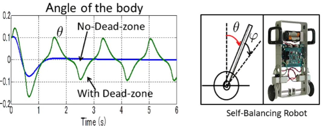
An example of the input dead-zone can be seen in the mechanism activated by a motor. In this thesis, we will treat the dead-zone in the motor wheel mechanism of a self-balancing robot as modeled an inverted pendulum. In Fig. 2.4, the angle of the bodyθof the self-balancing robot is shown for the case where dead-zone is completely cancelled, and it is not cancelled at all. The angle of the bodyθexhibits vibration when the input dead-zone in the self-balancing robot is not cancelled.

In this thesis, we consider a single-input and multi-output system which consists of a linear time-invariant part Pand an input dead-zone D_δ as shown in (2.1). As in [26], when we know the exact value ofδ, we can completely eliminate the dead- zone nonlinearityD_δby using its right inverse.

We take into consideration a feedback control system to use ˆD_δ as depicted in Fig. 2.6. In the control system, a feedback controller C is designed to stabilize P. In Fig. 2.6, r is the reference input, u is the control input, y is the measured output, respectively. Unlike the ideal case where the exact value ofδis available, it is difficult to cancelD_δ by ˆD_δcompletely in practical application. The cancelation error causes the steady-state vibration in the control system when P is unstable.

Then, we need to determine an appropriate valueδ in ˆD_δ to suppress the steady- state periodic motion in the control system.

Figure 2.4: The response of the angle of the body of the self-balancing robot when it has dead-zone and no dead-zone

Figure 2.5: A system with an input dead-zone

Figure 2.6: Configuration of a feedback control system with dead-zone compensa- tion

Chapter 3

Discrete-time Extremum Seeking Control for Periodic Steady-states

3.1 Discrete-time Extremum Seeking

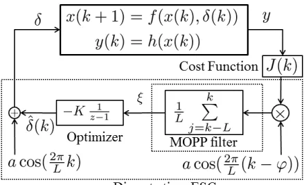
Extremum seeking control is known as a powerful adaptive method to optimize the control performance in real time. It is mainly used to optimize the control system with a constant steady-state output. In [8], an extremum seeking scheme for peri- odic steady-state outputs was proposed in the non-equilibrium case. In this thesis, we consider a discrete-time version of [8] which is summarized in Fig. 3.1. The fig- ure shows the configuration of a feedback control system with a tuning parameterδ connected with discrete-time extremum seeking control. We consider a plant as

x(k+1) = f(x(k), δ(k)) (3.1)

y(k) = h(x(k)). (3.2)

The extremum seeking control aims to tune the parameter δ to minimize the cost function of performance output [8] by given as

J(δ(k))=



1

N

∑k

i=k−N

y(i)²





1 2

(3.3) whereNis the period of the steady-state outputy. The extremum seeking scheme uses a perturbation (dither) signal

d₁(k)= acos2π

Lk (3.4)

with the periodL∈Zand an estimate ˆδof an optimal valueδ^∗by applying

δ(k)= δˆ(k)+d₁(k) (3.5)

to the system. We denote the estimation error by

δ˜(k)=δ^∗−δˆ(k) (3.6)

Figure 3.1: Discrete-time ESC scheme To use (3.5) and (3.6), we have

δ(k)=δ^∗−δ˜(k)+d1(k). (3.7) This perturbed signal affects (3.3). By applying the Taylor series expansion to (3.3), we have

J(δ(k)) = J(δ^∗−δ˜(k)+d1(k))

= J(δ^∗)+ ∂J

∂δ(δ^∗)[(δ^∗−δ˜(k)+d₁(k))−δ^∗]+ 1 2

∂²J

∂δ²[(δ^∗−δ˜(k)+d₁(k))−δ^∗]² J(δ^∗)+ ∂J

∂δ(δ^∗)(d2(k)−δ˜(k)+ 1 2

∂²J

∂δ²(δ^∗)(d2(k)−δ˜(k))², (3.8) where d₂(k) denotes the time delayed signal of d₁(k) due to the dynamics in the closed-loop system as

d₂(k)=acos2π

L (k−φ), φ∈Z. (3.9)

SinceJ(δ) is optimal atδ^∗, ^∂_∂δ^J(δ^∗)=0. Hence, J(δ(k)) J(δ^∗)+ 1

2

∂²J

∂δ²(δ^∗)(d₂(k)−δ˜(k))². (3.10) This cost function is multiplied by the demodulation signald2(k), and applied into a moving-average filter, also called a mean-over-perturbation-period (MOPP) filter, over the period ofd₂(k). Then, the output is

ξ(k)= 1 L

∑k

j=k−L

d2(j) (

J(δ^∗)+ 1 2

∂²J

∂δ²(δ^∗)(d2(k)−δ˜(k))² )

. (3.11)

By simple calculation, we have

∑k

j=k−L

d₂(j)=0,

∑k

j=k−L

d₂²(j)= a²L 2 ,

∑k

j=k−L

d³₂(j)= 0. (3.12) Hence, when we can assume that ˜δ(j) is constant over the periodL, we have

ξ(k)= −a² 2

∂²J

∂δ²(δ^∗)˜δ(k). (3.13) The signalξ(k) is used to generate the estimate ˆδby using the optimizer (the discrete- time integrator) as

δˆ(k)=−K 1

z−1ξ(k). (3.14)

Herezis the time-shift operator, that iszδˆ(k)=δˆ(k+1). Hence, (3.14) is equivalently δˆ(k+1)=δˆ(k)−Kξ(k). (3.15) To use (3.5) and (3.11), we can rewrite (3.15) as

δ˜(k+1) = δ˜(k)+Kξ(k)

= (

1−Ka² 2

∂²J

∂δ²(δ^∗) )

δ˜(k). (3.16)

Hence, we have next theorem.

Theorem 1.

If

1−Ka²

2

∂²J

∂δ²(δ^∗)

< 1, (3.17)

then an estimate ˆδconverges to the optimal valueδ^∗by extremum seeking. The con- vergence rate to the optimal value depends on the amplitudea of the perturbation signald1andd2, and the gainK of the optimizer. Since the Hessian ∂²J

∂δ²(δ^∗) of Jis unknown, we should start with small values foraandK to find appropriate values.

Moreover, the following underlying assumptions are also required [8], [12].

Assumption 1. For all fixed parameterδ over the range for tuning, the stabilized closed-loop system has a unique globally asymptotically stable steady-state solu- tion with a constant period.

Assumption 2. The cost function J(δ) has a unique global minimum at δ^∗ for steady-state performance.

We can illustrate the signals in discrete-time extremum seeking control in Fig. 3.2.

Firstly, (a) oscillation can be seen in the measured output signalyof the plant (b)

Figure 3.2: Process signals in the discrete-time extremum seeking control the cost function J (3.3) is calculated to use the output signaly. Secondly, (c) the oscilation in the outputydoes not appear in the cost function Jin the steady-state, then (d) J is multiplied by the demodulation signald₂ (3.9). Thirdly, (e) the de- modulated signal is filtered by (f) the MOPP filter to produce the output signal ξ (g). Futhermore, the output signal ξ gets in (h) the optimizer then the estimation of dead-zone compensation of the signal (i) add with the perturbation signald₁ (j).

Fourthly, the process signal of extremum seeking automatically updates the param- eter (k) until we get the optimal value which achieves zero of the output signal of MOPP filter and we can see reducing oscillation in the output measuredysignal (ℓ).

So, this process indicates effectively and successfully extremum seeking control for automatically tuning parameter to optimize the control performance.

3.2 Extremum Seeking Parameters Influence on Per- formance

The summarized algorithm for tuning dead-zone compensation by discrete-time ex- tremum seeking consists of

1. Design of a stabilizing controller for the closed-loop system,

2. Design of the cost function of the output measurement of the system,

3. Design parameters of extremum seeking such as frequency or period of pertur- bation or dither signal, MOPP filter, gain optimizer which check :

• Period of the outputy

• Output of the cost function signal with static or constant steady-state

• Assumption 1 and 2 are satisfied

• Convergence by Theorem 1

Futhermore, we can design and analyse how to choose properly parameters of ex- tremum seeking to tune dead-zone compensation for good performance and fast rejection dead-zone. The extent of the influence of parameters can be good perfor- mance if the parameters of extremum seeking are enlarged and reduced that will be further describe below.

• Gain of the optimizer K

Gain optimizerKadjusts the convergence speed and stability system.

• Phase of the perturbation signalφ

In [8], the phase of the perturbation signal selects the constantφ∈R≥0which is an estimate of the sum of the time-varying delay of the plant dynamics and the performance measure of cost function for a good chosen.

• Period of the perturbation L

Period of the perturbation signal L should be chosen larger than period of the cost function N. So, we check the output signal of cost function before designing period of the perturbation signal.

• Period of MOPP Filter L

Period of the MOPP filter is same with the period of the perturbation signal.

• Amplitude of the perturbation signal a

For designing the amplitude of the perturbation signal, we select small value which is smaller than cost function value in initial parameter without ex- tremum seeking.

3.3 Stability analysis

The stability of extremum seeking was first analyzed by Wang and Krsti`c [19]. They proposed averaging and singular perturbation to derive stability conditions of an extremum seeking feedback scheme [19] in which the averaging theorem adopted theorem 8.3 in Khalil as detail see [17] and Appendix C. To guarantee practical asymptotic stability, Teel et al. [25] proposed a generalized Lyapunov theorem.

Stability analysis of extremum seeking for periodic steady-state suggested by Haring et.al [8]. To apply extremum seeking, we used a stabilized controller which stabilize the plant of system which is a Discrete-Time Linear Quadratic Gaussian (LQG) controller to stabilize the closed-loop system. Stability of the closed loop system is ensured by appropriate state feedback gain and state estimation gain in LQG.

Chapter 4

Extremum Seeking for Dead-zone Compensation and Its Application to a Self-Balancing Robot

4.1 Self-Balancing Robot

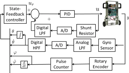
In this section, we use discrete-time extremum seeking control discussed in the pre- vious chapter to optimize a dead-zone compensation for the self-balancing robot which is a commercial product called e-nuvo WHEEL shown in Fig. 4.1. The feed- back controllerC for the self-balancing robot is initially designed to use the model based on dynamic equations and the catalog parameters, and secondly done to use the model obtained by closed loop identification.

4.2 Models of Self-Balancing Robot

4.2.1 Physical equation based model

The equation of motion of the self-balancing robot as an inverted pendulum can be described as

[(M+m)r²_t +J_t+mlr_tcosθ(t)+iJ_m]¨θ(t)−mlr_t(sinθ(t))˙θ²(t) (4.1) +[(M+m)r²_t +J_t +i²J_m] ¨φ+cφ˙ =ηi k_tu(t).

[(M+m)r_t²+ J_t+2mlr_tcosθ(t)+ml²+J_p+J_m]¨θ(t)−mlr_tsinθ(t)˙θ²(t) (4.2)

−mglsinθ(t)+[(M+m)r²_t +J_t +mlr_tcosθ(t)+iJ_m] ¨φ= 0 where physical parameters are defined in Table 4.1. When we assume that

sinθ(t)≈ θ, cosθ(t)≈ 1, θ˙²(t)≈ 0, (4.3) (4.1) and (4.2) can be rewritten by

[(M+m)r_t²+ J_t+iJ_m+mlr_t]¨θ(t) (4.4) +[(M+m)r²_t +J_t +i²J_m] ¨φ(t)+cφ˙(t)= ηi k_tu(t)

Figure 4.1: Modeling of the Self-balancing robot (ZMP Inc.)

[(M+m)r²_t +J_t +2mlr_t+ml²+J_p+J_m]¨θ (4.5)

−mglθ+[(M+m)r²_t +J_t+mlr_t +iJ_m] ¨φ =0

As in [27], the state space continuous-time model of the self-balancing robotP in Fig. 4.1 can be derived from physical equations as

˙

x(t) = A_cx(t)+B_cu(t) (4.6)

y(t) = C_cx(t) (4.7)

wherex = [θ φ θ˙ φ˙]^T consists of the angle of the bodyθ, the relative angle of the wheel to the bodyφ, the angular velocity of the body ˙θand the relative angular ve- locity of the wheel to the body ˙φ. The control inputuis electrical current. Together with Table 4.1 [27], [28], we haveA_c, B_cas

A_c =

[ 02×2 I2×2

−E⁻¹G −E⁻¹F ]

=







0 0 1 0

0 0 0 1

104.05 0 0 0.06

−341.64 0 0 −0.37





, B_c =

[ 0_2×2

−E⁻¹ζ ]

=







0 0 37.8

−232.7





,

(4.8) where

E =

[ e₁₁ e₁₂

e₂₁ e₂₂ ]

+(

(M+m)r²_t +Jt

)I2, F =

[ 0 c

0 0 ]

, G=

[ 0 0

−mgl 0 ]

, ζ =

[ ηi K_t

0 ]

(4.9)

e₁₁=e₂₂= mlr_t+iJ_m e₁₂=i²J_m

e₂₁=2mlr_t+ml²+J_p+J_m Since we measureφand ˙θ,

C_c =

[ 0 1 0 0 0 0 1 0

] .

Table 4.1: Parameters of Self-balancing robot

Mass of the cart (tire, draft shaft ,gear) [Kg] M 0.071

Mass of the body [Kg] m 0.5392

Moment of inertia of the body [Kg m²] Jp 2.160×10⁻³ Moment of inertia of the cart [Kg m²] J_t 8.632×10⁻⁵ Moment of inertia of motor rotor [Kg m²] Jm 1.30×10⁻⁷ Length between the wheel axle and gravity center of the body[m] l 0.1073

Radius of the wheel [m] r_t 0.02485

Friction of the wheel axle [Kg m²/s] c 1×10⁻⁴ Torque constant of the motor [N m/A] K_t 2.79×10⁻³

Reduction ratio of the gear i 30

Efficiency drive system η 0.75

4.2.2 Closed-loop Identification Model

We obtain measurement data of the self-balancing robot commercial product e- nuvo WHEEL and identify the state space model form the measurement data by MOESP-type closed-loop subspace model identification (CL-MOESP) [10], [11].

The obtained model is given by

A =









1.0033 −0.0298 0.0157 −0.0061 −0.0324 0.0079 0.9102 −0.2941 −0.0299 0.0013

−0.0030 0.1140 0.2547 −0.0970 0.0403

−0.0027 0.0123 −0.1012 1.0675 0.0177 0.0003 −0.0023 0.2437 0.0403 0.9341







, B =









−1.2453 0.3671

−0.1786 0.0710

−0.0063







, D=

[ −0.0108

0.0401 ]

,

C =

[ −0.0796 −0.2888 −0.0025 0.0075 −0.2407

0.0148 −0.2744 −0.8751 −0.1124 0.2605 ]

.

Figure 4.2: Experiment e-nuvo WHEEL scheme

4.3 Design of a Stabilizing Controller

To discretize the continuous-time model (4.1) and (4.2) by zero-order hold, we ob- tain the discrete-time model

x(k+1) = A x(k) + B u(k) (4.10)

y(k) = C x(k). (4.11)

When we use the sampling periodT_s= 0.01 sec, we have

A =







1 0 0.01 0

−0.02 1 −0.0001 0.01

1.04 0 1 0

−3.42 0 −0.02 1





, B=







0.002

−0.01 0.38

−2.32





, C = C_c.

The discrete-time model is used to design the discrete-time LQG controller [13], [22] in Fig. 4.3 which minimizes

E



lim

τ→∞

1 τ

∑τ

k=0

x^T(k)Qx(k)+u^T(k)Ru(k)



 (4.12)

where Q and R are given constant weight matrices for which Q = Q^T ≥ 0, R = R^T > 0, under the existence of the process noise and the measurement noise. We assumed weight matricesQ= I₄, R =1 and covariance of the process noiseW =1 and the measurement noiseV =0.012 I₂which means rms noise 1% on each sensor channel. The feedback gainKis derived as

K =(B^TS B+R)⁻¹B^TS A, (4.13) and the solutionS =S^T ≥0 of the associated Riccati equation

A^TS A−S −(A^TS B+N)(B^TS B+R)⁻¹(B^TS A+N^T)+Q=0. (4.14)

Figure 4.3: Discrete-time Linear Quadratic Gaussian control

The optimalLminimizingE[x(k)−x(k)]ˆ ^T[x(k)−x(k)] is given byˆ L=APC^T(CPC^T+ V)⁻¹ whereP = P^T ≥ 0 is the unique positive-semidefinite solution of discrete al- gebraic Riccati equation. The discrete-time linear quadratic Gaussian (LQG) con- troller is given by connecting the discrete-time linear quadratic regulator (LQR) and the discrete-time Kalman filter according to block diagram in Fig. 4.3.

4.4 Physical equation based Model

4.4.1 Dead-Zone Compensation

In the following, we set the actual dead-zone parameter δ = 2 for the numerical simulations. When we do not use the dead-zone compensator (this corresponds to δˆ = 0 in ˆD, the angle of the body θ shows periodic steady periodic steady-state motion with amplitude 0.1 rad (5.7 degree) as shown in Fig. 4.4 (a). On the other hand, when we use the dead-zone compensator ˆD_δwith ˆδ= 1, the amplitude of the periodic steady-state motion of the angle of the bodyθ is 0.05 rad (2.8 degree) as shown in Fig. 4.4 (b). Although the periodic steady-state motion is much reduced by the dead-zone compensator, it still remains due to the gap between the actualδ and ˆδin the dead-zone compensator. Hence, it is important to tune ˆδto suppress the periodic steady-state motion completely.

Figure 4.4: The angle of the body θ of the closed-loop system with dead-zone D_δ(δ = 2) (a) with no dead-zone compensator, (b) with dead-zone compensator Dˆ_δ(ˆδ =1)

4.4.2 Extremum Seeking for Tuning of Dead-Zone Parameter

For simplicity, we usey = θ for the output for extremum seeking control and the cost function

J(k)=



1

N

∑k

i=k−N

θ(i)²





1 2

whereas the output for feedback control is y = [φ θ˙]^T. The parameters for ex- tremum seeking control are as follows; the amplitude and the period of the pertur- bation signal are a = 1/16 and L = 1800, the gain of the optimizer isK = 3, the time delay of the perturbation signal ind₂ isφ = 100, the period of cost function isN = 180. The mean-over-perturbation-period can be implemented by a FIR fil- ter. A simulation result where tuning dead-zone compensation by the discrete-time ESC starts att = 200 sec is shown in Fig. 4.5 where x[0] = [0.01 0 0 0]^T as the initial variable. The dead-zone compensation parameter ˆδ converges to δ = 2.06 as shown in Fig. 4.5 (a). Although this final value is not the actual valueδ = 2, the periodic steady-state motion in the bodyθ is sufficiently suppressed as shown in Fig. 4.5 (b). Indeed, the cost function J decreases to sufficiently small value as shown in Fig. 4.5 (c). This result shows that the small gap between the dead-zone parameter compensation and the actual one is acceptable.

Figure 4.5: A simulation result when extremum seeking is applied for tuning of dead-zone compensator. (a) The tuned value of dead-zone compensator, (b) the angle of the body, (c) the cost function.

4.5 Simulation Results by CL-MOESP Identification Model

4.5.1 Dead-Zone Compensation

We applied the discrete-time LQG regulator to make stabilized unstabled plant from the CL-MOESP identification model of the Self-balancing robot because tuning by the discrete-time ESC was need stabilized plant. We utilized the discrete-time Kalman filter to estimation state and the discrete-time LQR to search state feedback gain. We used weight matrices Q = I₄,R = 1 and covariance of process noise W = 1 and measurement noise V = 0.01²I2 which means rms noise 1% on each sensor channel. Then we set dead-zone parameterδ = 2 and the initial state as by x₀ = [0.01 0 0 0]^T. So, we achieved simulation result of the CL-MOESP model of the closed-loop system without extremum seeking with dead-zone, dead-zone compensator and the discrete-time LQG regulator controller. When we utilize dead- zone D_δ = 2 and do not use the dead-zone compensator ˆD_δ = 0, the angle of the

Figure 4.6: The angle of the bodyθof CL-MOESP model of the closed-loop system with dead-zoneD_δ(δ = 2) (a) with no dead-zone compensator, (b) with dead-zone compensator ˆD_δ(ˆδ=1)

bodyθ shows periodic steady-state motion with amplitude 0.2 (11.46 degree) rad as shown in Fig. 4.6 (a). When, we use the dead-zone compensator ˆD_δwith ˆδ = 1, the amplitude of the periodic steady-state motion of the angle of the bodyθreduces to 0.05 rad (2.8 degree) as shown in Fig. 4.6 (b) for the CL-MOESP identification model.

4.5.2 Extremum Seeking for Tuning of Dead-Zone Parameter

We take the discrete-time ESC to tuning dead-zone compensation for rejecting vi- bration which is cost function from outputθby given

J(δ)=



1

N

∑k

i=k−N

θ(i)²





1 2

.

Afterward, we set extremum seeking parameters that are same with the previous setting of self-balancing robot derived physical equations model. Simulation result of the CL-MOESP model for tuning dead-zone compensation by the discrete-time ESC are shown in Fig. 4.7 with K = 3 and in Fig. 4.8 with K = 10 which are represented cost function of the CL-MOESP model J in Fig. 4.7 (a) is decrease to minimum, the angle of the body of the CL-MOESP model depict for rejection dead-zone and stabilized moving self-balancing robot in Fig. 4.7 (b), estimation dead-zone compensation ˆδthat is achieved 2 as fit as setting dead-zone it is shown in Fig. 4.7 (c) the tuned value of dead-zone compensator, but it needs time starting 200 second and achieved the optimal value after 500 second for K = 3 and after 250 second forK = 10. It has fastly convergence to optimal performance for gain optimizer K = 10 but it has negative value estimation delta around 210 second.

Afterthat, estimationξ( Fig. 4.7 (d) ) is zero. This indicates optimal performance.

Figure 4.7: Extremum seeking result when K = 3 for CL-MOESP model. Time response of (a) cost function (b) the angle of the body (c) tuned parameter (d) esti- mated gradient of the cost function

4.5.3 Analysis of Extremum Seeking Parameters

In Chapter 3, extremum seeking consists of four parameters which analyze the influ- ence of parameters can be good performance or not if the parameters of extremum seeking are enlarged or reduced that will be further describe below.

• Optimizer gain K

The optimiser gainK influences on the performance of the system as shown in Fig. 4.9 by the self-balancing robot CL-MOESP model. As results when we changed choose K = 1, 3, 10, 20, and 30 we show the cost function J in Fig. 4.10, output θ in Fig. 4.11, estimation delta ˆδ in Fig. 4.12 and ξ in Fig. 4.13. The performance when we use K = 10 is fastest to get optimal value about 50 second, but it has negative value around 210 second.

• Phase of perturbation signalφ

We select six phases of perturbation signalφthat areφ = 0.1, 1, 10, 30, 100 and 200. In Fig. 4.14, we show the simulation results for tuning dead-zone compensation by the CL-MOESP model, there are no significantly differences in the cost function J, estimation delta ˆδ, ξ and the angle of the body θ in Fig. 4.15.

• Period of perturbation signal L

Period L of the perturbation signal is chosen larger than period of the cost

Figure 4.8: Extremum seeking result whenK = 10 for CL-MOESP model. Time response of (a) cost function (b) the angle of the body (c) tuned parameter (d) esti- mated gradient of the cost function

function N. We select six variations of period of the perturbation signal which is N = 180 that consist of L = 1N, 5N, 10N, 20N, 30N, and 100N for analysis. It can be seen comparison period of perturbation signal Lwith the optimizer gain K = 3 and phase φ = 100 for the CL-MOESP model in Fig. 4.16. The outputθwith variation period of perturbation signalLcan be shown in Fig. 4.17. The best performance for variationLof simulation results of tuning dead-zone compensation by ES isL= 10N.

• Period of MOPP Filter L

For analysis of period of the MOPP filter, it has same with period of pertur- bation signal.

• Amplitude of perturbation signal a

To design the amplitude of the perturbation signal, we select a value which is smaller than the cost function value. For analysis, we choose the amplitude of the perturbation asa = 0.1134 from the cost function J = 0.1134 when the setting dead-zone d = 2 and without dead-zone compensation also with the optimizer gain K = 3, period of the perturbation L = 1800 and phase φ = 100. The variations ofa for analysis are 0.1a, 0.3a, 0.5a, 0.55a, aand 10a. The simulation results of tuning dead-zone compensation by ES with comparison the amplitude a of the perturbation signal for the CL-MOESP model represented in Fig. 4.18 and Fig. 4.19. It can be seen in Fig. 4.18 that

Figure 4.9: Comparison of optimizer gainKfor performance system of CL-MOESP model

it is not good result when we choose amplitude of perturbation signal with high value 10a. Hence, we should choose a value less than 1a. The value 0.55a is best because the cost function after 500 second approaches zero as in Fig. 4.20 and estimation ˆδ approaches an appropriate value around 550 second as in Fig. 4.21.

Figure 4.10: Comparison of optimizer gainK for performance of cost functionJof CL-MOESP model

Figure 4.11: Comparison of optimizer gain K for performance of outputθ of CL- MOESP model

Figure 4.12: Comparison gain optimizer K for performance of estimation delta ˆδof CL-MOESP model

Figure 4.13: Comparison gain optimizer K for performance of ξ of CL-MOESP model

Figure 4.14: Comparison of different phases of perturbation signalφ with the gain optimizerK = 3,(P=φ)

Figure 4.15: Comparison of the angle of the body θ with respect to variation of phase of the perturbation signalφwith gain optimizerK = 3,(P= φ)

Figure 4.16: Comparison of the periodLof the perturbation signal with phaseφ = 100 and the gain optimizerK =3

Figure 4.17: Comparison of the angle of the bodyθwith respect to the variation the periodLof perturbation signal with phaseφ=100 and the gain optimizerK = 3

Figure 4.18: Comparison of the amplitude aof perturbation signal with period of perturbationL= 1800, phaseφ=100 and the gain optimizer K =3

Figure 4.19: Comparison of the angle of the bodyθwith respect to the variation of the amplitudeaof perturbation signal with period of perturbationL = 1800, phase φ=100 and the gain optimizerK = 3

Figure 4.20: Comparison of the cost function J of amplitudeaof the perturbation signal

Figure 4.21: Comparison of estimation ˆδ of dead-zone parameter with respect to amplitudeaof the perturbation signal

Chapter 5 Conclusions

This dissertation describes a new techniques to compensate the dead-zone prop- erty in real time. Some conclusions as well as shortcomings and future works are presented.

5.1 Concluding Remarks

We conclude the dissertation as follows:

• In this dissertation, we proposed discrete-time extremum seeking control by the moving average filter to tune input dead-zone compensation in real time and applied it to the stabilized self-balancing robot with the dead-zone com- pensation.

• The effectiveness of the proposed method is illustrated by numerical sim- ulations. In the simulations, the compensation parameter converges to the optimal value minimizing the cost function of the performance output.

5.2 Future Works

We will evaluate the proposed discrete-time extremum seeking control for eliminat- ing dead-zone by an experiment using e-nuvo WHEEL. However, it is not easy to apply in real time by experiment because the running of experiment e-nuvo WHEEL is quickly while the process of tuning dead-zone parameters by computer needs time also transfer data from computer to e-nuvo WHEEL has time-delay. Therefore, we need to develop a method to rapidly process tuning dead-zone parameters through micro-controllerin e-nuvo WHEEL.

Appendix A

Model of Self-balancing Robot derived from physical equations

A.1 Modelling of Self-balancing Robot as Inverted Pendulum

The equation of motion of the self-balancing robot as an inverted pendulum can be described as

[(M+m)r²_t +J_t+mlr_tcosθ(t)+iJ_m]¨θ(t)−mlr_t(sinθ(t))˙θ²(t) (A.1) +[(M+m)r²_t +J_t +i²J_m] ¨φ+cφ˙ =ηi k_tu(t).

[(M+m)r_t²+ J_t+2mlr_tcosθ(t)+ml²+J_p+J_m]¨θ(t)−mlr_tsinθ(t)˙θ²(t) (A.2)

−mglsinθ(t)+[(M+m)r²_t +J_t +mlr_tcosθ(t)+iJ_m] ¨φ= 0 where physical parameters are defined in Table 4.1. When we assume that

sinθ(t)≈ θ, cosθ(t)≈ 1, θ˙²(t)≈ 0, (A.3) (A.1) and (A.2) can be rewritten by

[(M+m)r_t²+ J_t+iJ_m+mlr_t]¨θ(t) (A.4) +[(M+m)r²_t +Jt +i²Jm] ¨φ(t)+cφ˙(t)= ηi ktu(t)

[(M+m)r²_t +J_t +2mlr_t+ml²+J_p+J_m]¨θ (A.5)

−mglθ+[(M+m)r²_t +J_t+mlr_t +iJ_m] ¨φ =0 These two equations are combined into

E

[ θ¨

φ¨ ]

+F

[ θ˙

φ˙ ]

+G

[ θ

φ ]

=ζu, (A.6)

where E =

[ e₁₁ e₁₂

e₂₁ e₂₂ ]

+((M+m)r²_t +J_t)I₂, F =

[ 0 c

0 0 ]

, G=

[ 0 0

−mgl 0 ]

, ζ =

[ ηi k_t

0 ]

Figure A.1: Modeling of the Self-balancing robot

e₁₁=e₂₂= mlr_t+iJ_m (A.7)

e₁₂=i²J_m (A.8)

e₂₁=2mlr_t+ml²+J_p+J_m. (A.9)

From this second order differential equation, we have the state space model as

˙

x = A_cx(t)+B_cu(t) (A.10)

y(t) = C_cx(t) (A.11)

where

A_c =

[ 0_2×2 I_2×2

−E⁻¹G −E⁻¹F ]

, x=







φθ θ˙ φ˙





, B_c =

[ 0_2×2

E⁻¹ζ ]

C_c =







φθ θ˙ φ˙





.