RIMS-1718
Optimal matching forests and valuated delta-matroids
By
Kenjiro TAKAZAWA
March 2011
R ESEARCH I NSTITUTE FOR M ATHEMATICAL S CIENCES
KYOTO UNIVERSITY, Kyoto, Japan
Optimal matching forests and valuated delta-matroids
Kenjiro Takazawa
Research Institute for Mathematical Sciences, Kyoto University, Kyoto 606-8502, Japan.
[email protected] March 16, 2011
Abstract
The matching forest problem in mixed graphs is a common generalization of the matching problem in undirected graphs and the branching problem in directed graphs. Giles presented an O(n2m)-time algorithm for finding a maximum-weight matching forest, wheren is the number of vertices andmis that of edges, and a linear system describing the matching forest polytope.
Later, Schrijver proved total dual integrality of the linear system.
In the present paper, we reveal another nice property of matching forests: the degree se- quences of the matching forests in any mixed graph form a delta-matroid and the weighted matching forests induce a valuated delta-matroid. We remark that the delta-matroid is not necessarily even, and the valuated delta-matroid induced by weighted matching forests slightly generalizes the well-known notion of Dress and Wenzel’s valuated delta-matroids. By focusing on the delta-matroid structure and reviewing Giles’ algorithm, we design a simpler O(n2m)- time algorithm for the weighted matching forest problem. We also present a faster O(n3)-time algorithm by using Gabow’s method for the weighted matching problem.
1 Introduction
The concept of matching forestsin mixed graphs was introduced by Giles [14, 15, 16] as a common generalization of matchings in undirected graphs and branchings in directed graphs. Let G = (V, E, A) be a mixed graph with vertex set V, undirected edge set E and directed edge set A.
Let n and m denote |V| and |E ∪A|, respectively. For a vector x ∈ RE∪A and F ⊆ E ∪A, let x(F) :=∑
e∈F x(e).
We denote a directed edgea∈A fromu∈V tov∈V byuv. A directed edge is often called an arc. For an arc a=uv, the terminal vertex v is called thehead ofa and denoted by∂−a, and the initial vertexuis called the tailofaand denoted by∂+a. For a vertexv∈V, the set of arcs whose head (resp., tail) is v is denoted by δ−v (resp.,δ+v). For B ⊆A, let∂−B =∪
a∈B∂−a. A vertex in ∂−B is said to be covered by B. An arc subset B ⊆Ais a branchingif the underlying edge set of B is a forest and each vertexv ∈V is the head of at most one arc in B. For a branching B, a vertex not covered by B is called a root of B, and the set of the roots of B is denoted by R(B), i.e., R(B) =V \∂−B.
An undirected edgee∈E connectingu, v∈V is denoted by (u, v). We often abbreviate (u, v) as uv, where it obvious that it is undirected. Fore=uv∈E, both u and v are called as thehead of e, and the set of heads of e is denoted by ∂e, i.e., ∂e ={u, v}. For a vertex v, the set of edges incident to v is denoted byδv. ForF ⊆E, let∂F =∪
e∈F∂e. A vertex in∂F is said to becovered
by F. An undirected edge subsetM ⊆E is amatchingif each vertexv∈V is the head of at most one edge in M. A vertex not covered by M is called aroot of M and the set of the roots ofM is denoted by R(M), i.e.,R(M) =V \∂M.
An edge setF ⊆E∪A is amatching forestif the underlying edge set ofF is a forest and each vertex in V is the head of at most one edge inF. Equivalently, an edge set F = B∪M, where B ⊆AandM ⊆E, is a matching forest ifB is a branching andM is a matching with∂M ⊆R(B).
A vertex in ∂−B∪∂M are said to be covered byF, and a vertex is a root ofF if it is not covered by F. The set of the roots of F is denoted by R(F). Observe that R(F) = R(B)∩R(M) and V =R(B)∪R(M).
1.1 Background
Matching forests inherit the tractability of branchings and matchings. Let w∈RE∪A be a weight vector on the edge set of a mixed graph G = (V, E, A). We consider the weighted matching for- est problem, the objective of which is to find a matching forest F maximizing w(F). For this problem, Giles [15] designed a primal-dual algorithm running in O(n2m) time, which provided a constructive proof for integrality of a linear system describing the matching forest polytope.
Later, Schrijver [21] proved that Giles’ linear system is totally dual integral. These results com- monly extend the polynomial-time solvability and the total dual integrality results for the weighted branchings and weighted matchings [4, 7, 9].
Topics related to matching forests include the following. Using the notion of matching forests, Keijsper [17] gave a common extension of Vizing’s theorem [23, 24] on covering undirected graphs by matchings and Frank’s theorem [11] on covering directed graphs by branchings. Another aspect of matching forests is that they can be represented as linear matroid matching (see [22]). From this viewpoint, however, we do not fully understand the tractability of matching forests, since the weighted linear matroid matching problem is unsolved while the unweighted problem is solved [18].
In the present paper, we reveal a relation between matching forests anddelta-matroids [1, 3, 5]
to offer a new perspective on weighted matching forests which explains their tractability. For a finite set V and F ⊆ 2V, the pair (V,F) is a delta-matroid if it satisfies the following exchange property:
(DM) ∀S1, S2 ∈ F,∀s∈S1△S2,∃t∈S1△S2,S1△{s, t} ∈ F.
Here, △denotes the symmetric difference, i.e.,S1△S2 = (S1\S2)∪(S2\S1).
A typical example of a delta-matroid is amatching delta-matroid. For an undirected graphG= (V, E), letFM ={∂M |M is a matching in G}. Then, (V,FM) is a delta-matroid [2, 3]. Branch- ings in a directed graph also induce a delta-matroid, which we call a branching delta-matroid. For a directed graph G= (V, A), let FB ={R(B)|B is a branching inG}. Then, it is not difficult to verify that FB is a delta-matroid (see§ 2.1).
A delta-matroid (V,F) is called even if |S1| − |S2| is even for any S1, S2 ∈ F. Note that a matching delta-matroid is an even delta-matroid, whereas a branching delta-matroid is not. Even delta-matroids are characterized by the following simultaneous exchange property [25]:
(EDM) ∀S1, S2∈ F,∀s∈S1△S2,∃t∈(S1△S2)\ {s},S1△{s, t} ∈ F and S2△{s, t} ∈ F.
The concept of valuated delta-matroids [6, 26] is a quantitative generalization of even delta- matroids. A function f : 2V →R∪ {−∞}is a valuated delta-matroid if domf ̸=∅ and
(V-EDM) ∀S1, S2 ∈ domf, ∀s ∈ S1△S2, ∃t ∈ (S1△S2)\ {s}, f(S1△{s, t}) +f(S2△{s, t}) ≥ f(S1) +f(S2).
Here, domf := {S | S ⊆V,f(S)̸=−∞}. Note that (V,domf) is an even-delta matroid. We remark here that weighted matchings in a weighted undirected graph induce a valuated delta- matroid fM with domfM =FM (see §2.1).
1.2 Contributions
In this paper, we consider delta-matroids commonly extending matching delta-matroids and branch- ing delta-matroids, and also a valuation on those delta-matroids. For this purpose, we introduce a new class of delta-matroids which properly includes even delta-matroids. We call (V,F) asimulta- neous delta-matroid if it satisfies the following weaker simultaneous exchange property:
(SDM) ∀S1, S2∈ F,∀s∈S1△S2,∃t∈S1△S2,S1△{s, t} ∈ F and S2△{s, t} ∈ F.
Note that every even delta-matroid is a simultaneous delta-matroid. Also, a branching matroid is a simultaneous delta-matroid (see §2.1).
The first main result in this paper is that matching forests also induce a simultaneous delta- matroid. For a mixed graph G= (V, E, A), letFM F ={R(F)|F is a matching forest}. We prove that FM F is a simultaneous delta-matroid.
Theorem 1. For any mixed graph G= (V, E, A), it holds that (V,FM F) is a simultaneous delta- matroid.
Furthermore, we generalize the notion of valuated delta-matroids in order to deal with a quan- titative extension of Theorem 1. That is, we define valuated delta-matroids on simultaneous delta- matroids, which slightly generalize valuated delta-matroids on even delta-matroids [6]. We call a function f : 2V →R∪ {−∞} avaluated delta-matroid if domf ̸=∅and
(V-SDM) ∀S1, S2 ∈ domf, ∀s ∈ S1△S2, ∃t ∈ S1△S2, f(S1△{s, t}) +f(S2△{s, t}) ≥ f(S1) + f(S2).
Note that (V,domf) is a simultaneous delta-matroid.
For a weighted mixed graph (G, w) withG= (V, E, A) andw∈RE∪A, define a functionfM F : 2V →R∪ {−∞}by
fM F(S) =
{max{w(F)|F is a matching forest with R(F) =S} (S∈ FM F),
−∞ (otherwise).
We prove that fM F satisfies (S-VDM).
Theorem 2. For any weighted mixed graph (G, w), it holds thatfM F is a valuated delta-matroid.
Proofs for Theorems 1 and 2 will be given in § 2.2. We remark that the relation between valuated delta-matroids in the sense of [6] and those in our sense is similar to that between M-concave functions and M♮-concave functions [20].
The next contribution of this paper is new algorithms for the weighted matching forest problem:
we design a simpler algorithm and a faster algorithm than Giles’ algorithm [15]. In§ 3, we present a simple O(n2m)-time algorithm which focuses on the delta-matroid structure. We also present an O(n3)-time algorithm in § 4 by using the technique of Gabow [13] for the weighted matching problem.
2 Delta-matroids and matching forests
In this section, we prove Theorems 1 and 2. That is, we show relations between delta-matroids and matching forests, and between valuated delta-matroids and weighted matching forests.
2.1 Matching delta-matroids and branching delta-matroids
In this subsection, we describe basic facts on delta-matroids, including their relations to matchings and branchings. We begin with exhibiting two operations on delta-matroids. The dualof a delta- matroid (V,F) is a delta-matroid (V,F¯), defined by ¯F = {V \S | S ∈ F}. The union of two delta-matroids (V,F1) and (V,F2) is a pair (V,F1 ∨ F2) defined by F1 ∨ F2 = {S1 ∪S2 | S1 ∈ F1, S2∈ F2, S1∩S2 =∅}, which is a delta-matroid [2].
The relation between matchings and delta-matroids is well-known. Let (G, w) be a weighted undirected graph with G = (V, E) and w ∈ RE. As stated in § 1, the pair (V,FM), where FM ={∂M |M is a matching inG}, is an even delta-matroid, which we call the matching delta- matroid of G. Moreover, a function fM : 2V → R∪ {−∞} defined below is a valuated delta- matroid [19]:
fM(S) = {
max{w(M)|M is a matching with ∂M =S} (S∈ FM),
−∞ (otherwise).
We now present a relation between branchings and delta-matroids. Let (G, w) be a weighted directed graph withG= (V, A) andw∈RA. Recall thatFB ={R(B)|B is a branching inG}. It is verified that (V,FB) is a delta-matroid as follows. For a directed graph G, a strong component is called asource componentif it has no arc entering from other strong components. The vertex set and arc set of a strong component K are denoted byV K and AK, respectively. LetK1, . . . , Kl be all source components in G. Then, we have thatFB={S |S ⊆V,|S∩V Ki| ≥1 for i= 1, . . . , l}. Thus, it follows that (V,FB) is a generalized matroid [12]. Moreover, it also follows that (V,FB) satisfies (SDM). We call (V,FB) as the branching delta-matroid ofG.
Theorem 3. For any directed graphG, it holds that(V,FB) is a simultaneous delta-matroid.
Furthermore, this fact extends to weighted branchings. Define fB: 2V →R∪ {−∞}by fB(S) =
{
max{w(B)|B is a branching with R(B) =S} (S∈ FB),
−∞ (otherwise).
Then, fB is a valuated delta-matroid, which immediately follows from arguments in Schrijver [21, Theorem 1].
Theorem 4. For any weighted directed graph (G, w), it holds thatfB is a valuated delta-matroid.
2.2 Delta-matroids and matching forests
In this subsection, we prove Theorems 1 and 2. We begin with a simple proof showing that (V,FM F) is a delta-matroid for a mixed graph (V, E, A). Let FM be the matching delta-matroid of (V, E) and FB the branching delta-matroid of (V, A). Then, it immediately follows from the definition of matching forests that FM F is the dual of FM∨F¯B, and thus (V,FM F) is a delta-matroid.
We now prove Theorem 1, which is a stronger statement. First, Schrijver [21] proved the following exchange property of branchings.
Lemma 5 (Schrijver [21]). Let G = (V, A) be a directed graph, and B1 and B2 be branchings partitioning A. Let R1 and R2 be vertex sets with R1 ∪R2 = R(B1) ∪R(B2) and R1 ∩R2 = R(B1)∩R(B2). ThenA can be split into branchingsB′1 andB2′ withR(Bi′) =Ri fori= 1,2 if and only if each source component K in G satisfies that |K∩Ri| ≥1 for i= 1,2.
By using Lemma 5, Schrijver proved an exchange property of matching forests [21, Theorem 2].
Here, we show another exchange property of matching forests, which relates them to simultane- ous delta-matroids. The proof below is quite similar to the proof for Theorem 2 in [21]. For completeness, however, we describe a full proof.
Lemma 6. Let G= (V, E, A) be a mixed graph,F1 andF2 be matching forests partitioning E∪A, and s∈ R(F2)\R(F1). Then, there exist matching forests F1′ and F2′ which partition E∪A and satisfy one of the following:
(i) R(F1′) =R(F1)∪ {s} and R(F2′) =R(F2)\ {s},
(ii) R(F1′) =R(F1)∪ {s, t} and R(F2′) =R(F2)\ {s, t} for some t∈R(F2)\(R(F1)∪ {s}), (iii) R(F1′) = (R(F1)∪ {s})\ {t} andR(F2′) = (R(F2)\ {s})∪ {t} for some t∈R(F1)\R(F2).
Proof. LetMi:=Fi∩E andBi:=Fi∩Afori= 1,2. Denote the family of the source components in (V, A) by K. If v ∈ R(B1)∩R(B2) for v ∈ V, then we have {v} ∈ K. Thus, for a source component K ∈ Kwith |K| ≥2,K∩R(B1) andK∩R(B2) are not empty and disjoint with each other. For each K ∈ K with|K| ≥2, choose a pair eK of vertices, one of which is in K∩R(B1) and the other in K∩R(B2). DenoteN ={eK |K∈ K}. Note that N is a matching.
Construct an undirected graphH = (V, M1∪M2∪N). We have thatHis a disjoint collection of paths and cycles. For, an endpointuof an edgeeK ∈N satisfies that eitheru∈∂−B1oru∈∂−B2, and thus u is not covered by both of M1 and M2. Moreover, we have that s is an endpoint of a path P in H. For, since s∈ R(F2), we have that s is not covered by M2. If s is covered byM1, then s∈R(B1), and thuss∈R(B1)∩R(B2). This implies that sis not covered byN.
Denote the set of vertices on P by V P, the set of edges in M1 ∪M2 on P by EP, and let M1′ :=M1△EP andM2′ :=M2△EP. Then, both M1′ and M2′ are matchings and
R(M1′) = (R(M1)\V P)∪(R(M2)∩V P), R(M2′) = (R(M2)\V P)∪(R(M1)∩V P).
Now, by Lemma 5, there exist disjoint branchings B1′ and B2′ such that
R(B′1) = (R(B1)\V P)∪(R(B2)∩V P), R(B2′) = (R(B2)\V P)∪(R(B1)∩V P).
(Note that |K∩R(Bi′)| ≥1 fori= 1,2 for every source component K.)
Since R(Bi)∪R(Mi) =V, we have thatFi′ :=Bi′∪Mi′ is a matching forest for i= 1,2, and R(F1′) = (R(F1)\V P)∪(R(F2)∩V P), R(F2′) = (R(F2)\V P)∪(R(F1)∩V P).
If V P = {s}, then Assertion (i) applies. Otherwise, denote the other endpoint of P by t. If t∈V \(R(F1)△R(F2)), then Assertion (i) applies. Ift∈R(F2)\R(F1), then Assertion (ii) applies.
If t∈R(F1)\R(F2), then Assertion (iii) applies.
Theorem 1 is obvious from Lemma 6. Furthermore, Theorem 2 also follows from Lemma 6.
Proof for Theorem 2. Let S1, S2 ∈domf and s∈S1△S2. Fori= 1,2, letFi be a matching forest such thatR(Fi) =Si and w(Fi) =fM F(Si). Without loss of generality, assumes∈R(F2)\R(F1).
By applying Lemma 6 to the mixed graph consisting of the edges inF1 andF2, we obtain matching forestsF1′ andF2′ such thatw(F1′)+w(F2′) =w(F1)+w(F2) and satisfying one of Assertions (i)–(iii).
Now the statement follows from w(F1′)≤fM F(R(F1′)) andw(F2′)≤fM F(R(F2′)). □
3 A simpler algorithm
Let (G, w) be a weighted mixed graph with G = (V, E, A) and w ∈ RE∪A. In this section, we describe a primal-dual algorithm for finding a matching forestF maximizingw(F). This algorithm is a slight modification of Giles’ algorithm [15]. The main difference results from focusing the delta-matroid structure of branchings (Theorem 3).
3.1 LP formulation for the weighted matching forest problem For a subpartition L of V, let ∪Ldenote the union of the sets inL and let
γ(L) :={e|e∈E,eis contained in∪L} ∪ {a|a∈A,ais contained in some set in L}.
LetΛ denote the collection of subpartitionL ofV with|L|odd. The following is a linear program- ming relaxation of an integer program describing the weighted matching forest problem:
(P) maximize ∑
e∈E∪A
w(e)x(e)
subject to x(δhead(v))≤1 (v∈V), (1)
x(γ(L))≤ ⌊| ∪ L| − |L|/2⌋ (L ∈Λ), (2)
x(e)≥0 (e∈E∪A). (3)
Here, δhead(v) ⊆ E ∪A denotes the set of edges which have v as a head, i.e., δhead(v) = δv∪ δ−v. Note that the above linear system is a common extension of those describing the weighted matching problem [7] and the weighted branching problem [9]. Giles [15] proved the integrality of the system (1)–(3).
Theorem 7 ([15]). For any weighted mixed graph (G, w), the linear program (P) has an integer optimal solution.
Furthermore, Schrijver [21] proved that the system (1)–(3) is totally dual integral [10], which commonly extends the total dual integrality of those for matchings [4] and for branchings. That is, Schrijver proved that the following dual problem of (P) has an integer optimal solution if w is integer:
(D) minimize ∑
v∈V
y(v) +∑
L∈Λ
z(L)⌊| ∪ L| − |L|/2⌋ subject to y(u) +y(v) + ∑
L:e∈γ(L)
z(L)≥w(e) (e=uv ∈E), (4) y(v) + ∑
L:a∈γ(L)
z(L)≥w(a) (a=uv ∈A), (5)
y(v)≥0 (v∈V), (6)
z(L)≥0 (L ∈Λ). (7)
Theorem 8 ([21]). For any weighted mixed graph (G, w) with w integer, the linear program (D) has an integer optimal solution.
Define the reduced weight w′∈RE∪A by w′(e) =y(u) +y(v) + ∑
L:e∈γ(L)
z(L)−w(e) (e=uv ∈E), w′(a) =y(v) + ∑
L:a∈γ(L)
z(L)−w(a) (a=uv ∈A).
Below are the complementary slackness conditions of (P) and (D).
x(e)>0 =⇒ w′(e) = 0 (e∈E∪A), (8)
x(δheadv)<1 =⇒ y(v) = 0 (v ∈V), (9) z(L)>0 =⇒ x(γ(L)) =⌊| ∪ L| − |L|/2⌋ (L ∈Λ). (10) 3.2 Algorithm description
3.2.1 Notations
In the algorithm, we keep a matching forest F, which corresponds to an integer feasible solution x of (P), and a dual feasible solution (y, z). We maintain thatx and (y, z) satisfy (8) and (10). The algorithm terminates when (9) is satisfied.
Similarly to the classical weighted matching and branching algorithms, we execute shrinking of subgraphs repeatedly. We keep two laminar families ∆and Υ of subsets of V, the former of which results from shrinking a strong component in the directed graph and the latter from shrinking an undirected odd cycle.
We use the following notations to describe the algorithm.
• For a cycle or a pathQ in an undirected graph (V, E), let V Qand EQdenote the vertex set and edge set of Q, respectively. We often abbreviateEQasQ.
• Ω′ :=∆∪Υ, Ω:=Ω′∪ {{v} |v∈V}.
• For eachU ∈Ω′, letGU = (VU, EU, AU) denote the mixed graph obtained from the subgraph induced by U by contracting all maximal proper subsets of U belonging to ∆. Also, let Gˆ = ( ˆV ,E,ˆ A) denote the mixed graph obtained fromˆ G by contracting all maximal sets in Ω′. We denote a vertex in a shrunk graph by the set of vertices in V which are shrunk into the vertex. Also, we often identify a vertex U in a shrunk graph and the singleton{U}.
• For G= (V, E, A) and a dual feasible solution (y, z), the equality subgraph G◦ = (V, E◦, A◦) of G is a subgraph defined by E◦ ={e|e∈E,w′(e) = 0} and A◦ ={a|a∈A,w′(a) = 0}.
We denote the branching delta-matroid in ( ˆV ,Aˆ◦) by ( ˆV ,FˆB◦), i.e., FˆB◦ ={R( ˆB)|Bˆ⊆Aˆ◦ is a branching in ˆG◦}. The outline of the algorithm is as follows.
• We maintain a matching forest ˆF = ˆM∪Bˆ in ˆG◦, where ˆM ⊆Eˆ◦ and ˆB ⊆Aˆ◦, in order to maintain (8).
• In contracting a vertex set U ⊆V, we associate a partition LU of U such thatx(γ(LU)) =
⌊| ∪ LU| − |LU|/2⌋. The vector z is restricted to subpartitions associated to the sets inΩ′ in order to maintain (10).
a v
a v
u u
w w
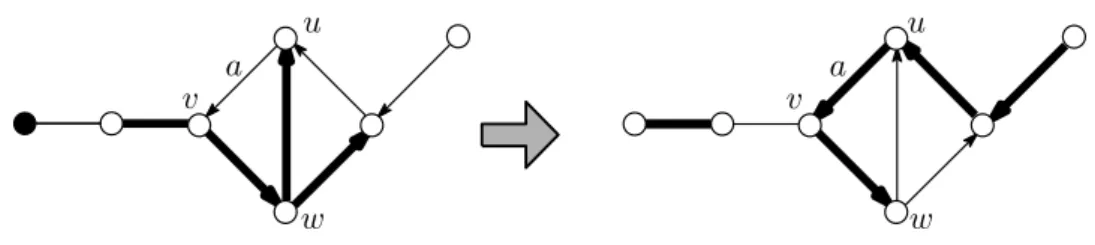
Figure 1: Augmentation. (Thick edges are in ˆF and the black vertex is a source vertex.)
• Similarly to Edmonds’ matching algorithm [8], we construct an alternating forest H, which is a subgraph of ( ˆV ,Eˆ◦). The vertex set and edge set of H are denoted by ˆV H and ˆEH, respectively. We often abbreviate ˆEH as H. Each component ofH is a tree and contains a unique source vertex. Intuitively, a source vertex is a vertex where (9) is not satisfied (see
§ 3.2.3 for precise definition). For v ∈V H, letˆ Pv denote the path in H connecting a source vertex and v. The edges incident to a source vertex does not belong to ˆM, and edges in ˆM and ˆE◦\Mˆ appear alternately on each Pv. We label a vertex v as “even” (resp., “odd”) if the length of Pv is even (resp., odd). Here, the length of a path is defined by the number of its edges. The set of vertices labelled as even (resp., odd) is denoted by even(H) (resp., odd(H)). Also, let free(H) := ˆV \(even(H)∪odd(H)).
3.2.2 A rough description of augmentation and shrinking
Before presenting a full description of the algorithm, we briefly sketch how to augment the matching forest, shrink subgraphs and associate a partition with the shrunk vertex set.
To make things easy, let us suppose that no subgraph is shrunk, i.e., ∆=Υ =∅ and ˆG=G.
Denote the current matching forest by ˆF = ˆM∪Bˆ, where ˆM ⊆Eˆ◦ is a matching and ˆB⊆Aˆ◦ is a branching.
After labeling a vertex v as even in growing the alternating forest H, we search for an arc a∈ Aˆ◦∩δ−v. Note that arcs in δ−v do not belong to ˆB. If such an arc a is found, our algorithm proceeds as follows.
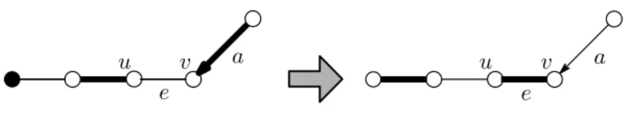
• If R( ˆB)\ {v} ∈ FˆB◦, then reset the matching forest ˆF := M′ ∪B′, where M′ := ˆM△Pv and B′ is a branching in ( ˆV ,Aˆ◦) with R(B′) = R( ˆB)\ {v}. This procedure is one kind of augmentation, in which the number of vertices violating (9) decreases. See Figure 1 for an illustration.
• If R( ˆB)\ {v} ̸∈ FˆB◦, it follows that v ∈ V Kˆ for some source component K of ( ˆV ,Aˆ◦) and V Kˆ \ {v} ⊆∂−Bˆ. IfK contains no undirected edge in ˆE◦, we addX= ˆV K to∆and update Gˆ by contracting the vertices in X to a single vertex. The newly created vertex is called a pseudo-vertex, denoted by X ∈ Vˆ. We then define a partition LX of X by LX ={X} and set z(LX) = 0. Note that (10) holds for LX, since x(γ(LX)) = |X| −1, | ∪ LX|=|X|and
|LX|= 1. See Figure 2 for an illustration. The case where K contains an undirected edge in Eˆ◦ will be described in §3.2.3.
Note that we can determine whether R( ˆB)\ {v} ∈FˆB◦ or not by decomposing ( ˆV ,Aˆ◦) into strong components. Also, it is not difficult to find a branching B′ ⊆Aˆ◦ withR(B′) =R(B)\ {v}.
Remark 9. The above bifurcation is the main difference from Giles’ algorithm [15]. In Giles’
algorithm, we augment the matching forest if B′′ = ˆB ∪ {a} is a branching in ˆG, which is a
a
v X
Figure 2: Shrinking of a source component. (Thick edges are in ˆF and the black vertex is a source vertex. The square in the shrunk graph indicates the pseudo-vertex X ∈Vˆ.)
u e v
u e v
Figure 3: Augmentation. (Thick edges are in ˆF and the black vertex is a source vertex.) sufficient condition for R( ˆB)\ {v} ∈FˆB◦. (Here, we reset the matching forest ˆF := M′∪B′′.) If B′′ is not a branching, we have that B′′ contains exactly one directed cycle D, and we contract X′ = V D to a single vertex. For instance, in Figure 1 we do not augment ˆF but contract the directed cycle consisting of u, v, w in Giles’ algorithm.
Also, if we find an undirected edgee∈Eˆ◦ connecting two even vertices uand v, we do similar procedures as the the classical blossom algorithm [8]. If u andv belong to different components in H, then we augment the matching forest by resetting ˆF :=M′∪B, whereˆ M′:=M△(Pu∪Pv∪{e}).
See Figure 3 for an illustration.
Assume that u and v belong to the same component of H (see Figure 4 for an illustration).
Here,H∪{e}contains exactly one odd undirected cycleC. We now add U = ˆV C toΥ, and update Gˆ by contracting the vertices inU to a pseudo-vertexU ∈Vˆ. We then define a partition LU of U by LU ={{v} |v∈U}and set z(LU) = 0. Note that (10) holds for LU, sincex(γ(LU)) =⌊|U|/2⌋ and | ∪ LU|=|LU|=|U|.
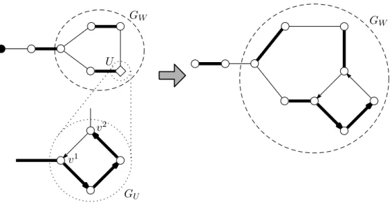
Dealing with a subgraph containing pseudo-vertices is a bit more complicated. Consider shrink- ing a source componentKin ˆGand letX⊆V be the union of vertices in ˆV K. Denote the maximal proper subsets of X belonging to ∆ and Υ by Y1, . . . , Yk ∈ ∆ and W1, . . . , Wl ∈ Υ, respectively.
Here, we can assume that arcs in ˆAK∩(δ+Wi∪δ−Wi) are incident to an identical vertexvWi ∈VWi
for every i= 1, . . . , l, since otherwise we can augment the current matching forest (see Figure 5).
LetX′ = (X\(W1∪ · · · ∪Wl))∪ {vW1} ∪ · · · ∪ {vWl}. Note thatX′ forms the vertex set of a strong component in (V, A◦). We now add X′ to∆ and let LX′ ={X′} be the associated partition with
u e v
U
Figure 4: Shrinking of an undirected odd cycle. (Thick edges are in ˆF and the black vertex is a source vertex. The pentagon in the shrunk graph indicates the pseudo-vertex U ∈Vˆ.)
a
v W
f+
f−
f+
f−
GW
f+
f−
GW
a
v W
f+
f−
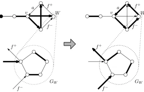
Figure 5: Augmentation. (Thick edges are in ˆF and the black vertex is a source vertex. The graph inside the dotted circle indicates GW, which is shrunk into the vertex W in ˆG◦.)
X′. See Figure 6 for an illustration.
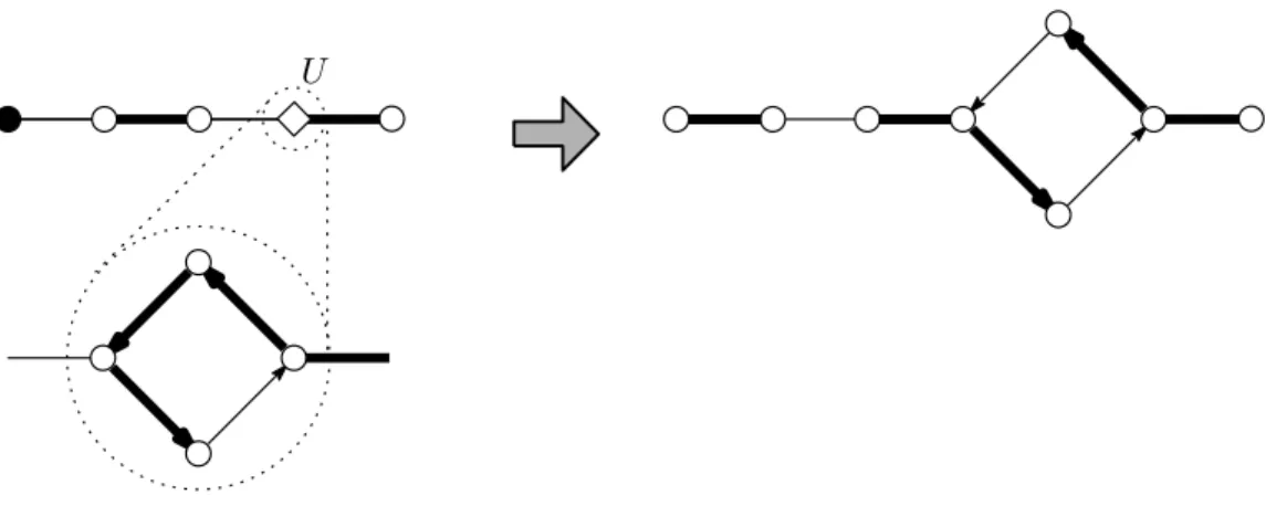
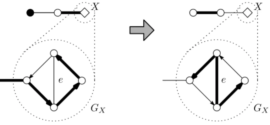
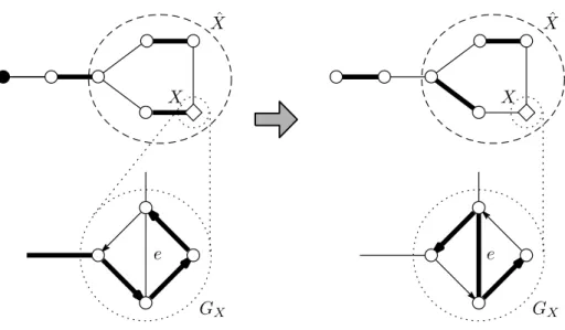
Finally, consider shrinking an odd undirected cycle C. Let U ⊆V denote the union of vertices in ˆV C. Denote the maximal proper subsets of U belonging to∆by Y1. . . , Yk∈∆and the proper subsets of U belonging toΥ W1. . . , Wl∈Υ, respectively. LetCU be an odd cycle inGU which can be obtained by adding even number of edges from each EWj toC. Fori= 1, . . . , k, letfi1, fi2 ∈CU denote the two edges incident to Yi, and let v1i, vi2 ∈Yi denote the vertices to whichfi1 and fi2 are incident, respectively. If, for some Yi, the two vertices vi1 and v2i are distinct and z(LYi′) = 0 for the minimal subset Yi′ ∈ ∆ of Yi such that {vi1, vi2} ⊆ Yi′, we can augment the current matching forest (see Figure 7 for an illustration).
Suppose otherwise. Without loss of generality, assume that vi1 and vi2 are identical for i = 1, . . . , j, and distinct for i = j + 1, . . . , k. For i = j + 1, . . . , k, let Yi′ ∈ ∆ be the minimal subset of Yi such that {v1i, vi2} ⊆ Yi′. Note that z(LYi′) > 0 for i = j+ 1, . . . , k. Let U′ = (U\(Y1∪· · ·∪Yk))∪{vY1, . . . , vYj}∪(Yj+1′ ∪· · ·Yk′). We now addU′ toΥ, and define a partitionLU′
of U′ by the collection of {vY1}, . . . ,{vYj}, Yj+1′ , . . . , Yk′ and singletons of the other vertices in U′. See Figure 8 for an illustration.
3.2.3 A full description of the algorithm We now present a full description of our algorithm.
Algorithm SIMPLE
Input. A weighted mixed graph (G, w), where G= (V, E, A) and w∈RE∪A. Output. A matching forestF inGmaximizing w(F).
Step 1. Set F :=∅, y(v) := max{{w(e)/2|e∈E},{w(a) |a∈A}} for every v ∈V,∆:= ∅and Υ :=∅. (Hence Ω={{v} |v∈V}, ˆG=G, ˆF =∅and z is void.)
Step 2. Construct the equality subgraph ˆG◦ = ( ˆV ,Eˆ◦,Aˆ◦). Define the set of source vertices ˆS = {U |U ∈Vˆ,y(v)>0 and x(δhead(v)) = 0 for somev∈U}. If ˆS = ∅, deshrink every sets in
Y W1
W2 vW2
vW1
X′
Figure 6: The graph on the left is a strong component K in ˆG, whereY ∈∆andW1, W2 ∈Υ. The graph on the right represents a graph obtained by deshrinkingY,W1 andW2. The dotted squares indicate X′, which is newly added to ∆.
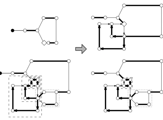
Figure 7: The two graphs above are ˆGand those below areG. The dotted box indicatesW ∈Υ and the nested three dashed boxes indicateY, Y′, Y′′ ∈∆, whereY′′⊆Y′ ⊆Y andz(LY′) =z(LY) = 0.
In the present step, augmentation and deshrinking of Y and Y′ are executed.
Y2
Y1
W
vY1 Y2′
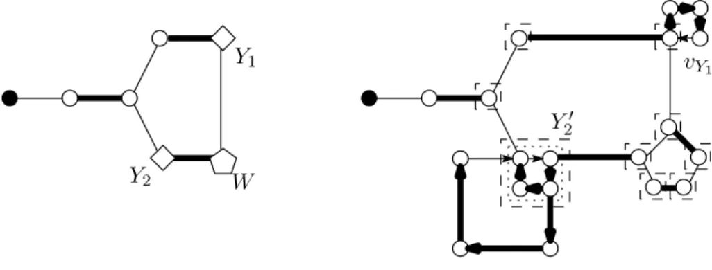
Figure 8: The graph on the left is an odd cycle C in ˆG, where Y1, Y2 ∈∆and W ∈Υ. The graph in the right represents G, where the dotted box indicates Y2′ with z(LY2′)>0. The set of vertices inside the dashed boxes is U′, where the dashed boxes indicate the partition LU′.
a v e
a v e
Figure 9: Augmentation in Step 4.2.1. (Thick edges are in ˆF and the black vertex is a source vertex.)
Ω′ and returnF. Otherwise, letH be ( ˆS,∅), label the vertices in ˆS as even, and then go to Step 3.
Step 3. If there exists an arc a∈Aˆ◦\Bˆ with∂−a∈ even(H), then go to Step 4. Otherwise, go to Step 5.
Step 4. Let v:=∂−a. IfR( ˆB)\ {v} ∈FˆB◦, then go to Step 4.1. Otherwise, go to Step 4.2.
Step 4.1: Augmentation. Reset ˆF := M′∪B′, where M′ := ˆM△Pv and B′ is a branching in ( ˆV ,Aˆ◦) withR(B′) =R( ˆB)\ {v}. Delete eachT ∈Ω′ with z(LT) = 0 from Ω′, and then go to Step 2. See Figure 1 for an illustration.
Step 4.2. LetK be the source component containing v and letX⊆V be the union of vertices in V Kˆ .
• If there exists e∈Eˆ◦\Mˆ such that∂e⊆V K, then go to Step 4.2.1.ˆ
• Otherwise, go to Step 4.2.2.
Step 4.2.1: Augmentation. LetBKbe a branching inKwithR(BK) =∂e. Reset ˆF :=M′∪B′, where M′ := ( ˆM△Pv)∪ {e} and B′ := ( ˆB \AK)ˆ ∪BK, delete each T ∈Ω′ withz(LT) = 0 from Ω′, and then go to Step 2. See Figure 9 for an illustration.
Step 4.2.2. Let W1, . . . , Wl be the maximal proper subsets of X belonging to Υ. If, for some i ∈ {1, . . . , l}, ˆAK contains a pair of arcs f+ ∈δ+Wi and f− ∈ δ−Wi such that ∂+f+ and
∂−f−belong to distinct vertices inGWi, then go to Step 4.2.2.1. Otherwise, go to Step 4.2.2.2.
Step 4.2.2.1: Augmentation. LetBK be a branching inK such thatR(BK) ={Wi} andf+∈ BK. Reset ˆF := M′ ∪B′, whereM′ := ˆM△Pv and B′ := ( ˆB\A(K))ˆ ∪BK∪ {f−}. Then, delete eachT ∈Ω′ withz(LT) = 0 fromΩ′ and go to Step 2. See Figure 5 for an illustration.
Step 4.2.2.2: Shrinking. For each i= 1, . . . , l, let vWi ∈VWi denote the unique vertex in GWi to which arcs in ˆAK are incident. LetX′ = (X\(W1∪ · · · ∪Wl))∪ {vWi} ∪ · · · ∪ {vWl} and add X′ to∆. LetLX′ ={X′} be the associated partition withX′, setz(LX′) := 0, and then go to Step 3. See Figure 6 for an illustration.
Step 5. Choose an edge e∈Eˆ◦\EHˆ such that one of its head u is even. Denote the other head of eby v.
• If v∈even(H) and econnects different components inH, then go to Step 5.1.
• If v∈even(H) and u and v belong to the same component inH, then go to Step 5.2.
• If v∈free(H) andv=∂−afor somea∈B, then go to Step 5.3.ˆ
• If v∈free(H) andv∈∂e′ for somee′ ∈Mˆ, then go to Step 5.4.
• If v is a pseudo-vertex labelled as “saturated,” then go to Step 5.5.
If no edge in ˆE◦\E(H) satisfies the above conditions, then go to Step 6.ˆ
Step 5.1: Augmentation. Reset ˆF := M′ ∪B, whereˆ M′ := ˆM△(Pu ∪Pv ∪ {e}), delete each T ∈Ω′ with z(LT) = 0 fromΩ′, and then go to Step 2. See Figure 3 for an illustration.
Step 5.2. LetCbe the cycle inH∪{e}and letU ⊆V be the union of the vertices in ˆV C. Denote the maximal proper subsets ofU belonging to∆andΥ byY1, . . . , Yk∈∆andW1. . . , Wl∈Υ.
Let CU be an odd cycle in GU obtained by adding even number of edges from each EWj to C. For i= 1, . . . , k, let fi1, fi2 ∈ CU denote the two edges incident to Yi, and let vi1, vi2 ∈Yi
denote the vertices to which fi1 and fi2 are incident, respectively. If, for some Yi, the two vertices vi1 and vi2 are distinct andz(LYi′) = 0 for the minimal subsetYi′ ∈∆ofYi such that {v1i, vi2} ⊆Yi′, then go to Step 5.2.1. Otherwise, go to Step 5.2.2.
Step 5.2.1: Deshrinking and augmentation. Delete Yi′ from ∆and reset Mˆ :=
{
( ˆM△PYi)△C (fi1, fi2 ∈E\M), M△Pˆ Y∗i (otherwise).
Here,PY∗
i denotes the path inH∪ {e}from ˆStoYi consisting of odd number of edges. Delete each T ∈Ω′ withz(LT) = 0 fromΩ′, and then go to Step 2. See Figure 7 for an illustration.
Step 5.2.2: Shrinking. Without loss of generality, assume that v1i and vi2 are identical for i = 1, . . . , j, and distinct fori=j+1, . . . , k. Fori=j+1, . . . , k, letYi′ ∈∆be the minimal subset ofYi such that{v1i, vi2} ⊆Yi′. LetU′ = (U\(Y1∪ · · · ∪Yk))∪ {vY1, . . . , vYj} ∪(Yj+1′ ∪ · · · ∪Yk′).
AddU′toΥ, and define a partitionLU′ofU′by the collection of{vY1}, . . . ,{vYj}, Yj+1′ , . . . , Yk′ and singletons of the other vertices in U′. See Figure 8 for an illustration.
Step 5.3: Augmentation. Reset ˆF := ( ˆM△Pv)∪( ˆB\ {a}), delete each T ∈Ω′ withz(LT) = 0 from Ω′, and then go to Step 2. See Figure 10 for an illustration.
Step 5.4: Forest extension. GrowH by adding eand e′. Labelvas odd and the other head of e′ as even. Then, go to Step 3.
u v u v e
a
e
a
Figure 10: Augmentation in Step 5.3. (Thick edges are in ˆF and the black vertex is a source vertex.)
Step 5.5: Augmentation. Reset ˆF :=M′∪B, whereˆ M′:= ˆM△Pv, and unlabel v. Delete each T ∈Ω′ with z(LT) = 0 and then go to Step 2.
Step 6. Apply Dual Update described below, delete each T ∈ Ω′ with z(LT) = 0 from Ω′, and then go to Step 3.
Procedure Dual Update. Define families of vertex subsets of V as follows:
∆+:={maximal set in ∆, contained in some even vertex},
∆−:={maximal set in ∆, contained in some odd vertex}, Υ+:={maximal set in Υ, contained in some even vertex}, Υ−:={maximal set in Υ, contained in some odd vertex}. Moreover, let
∆′+:={X ⊆V |X∈∆, maximal proper subset of some element in Υ+},
∆′−:={X ⊆V |X∈∆, maximal proper subset of some element in Υ−}, V+:={v∈V | {v} ∈even(H) or v is contained in some even vertex}, V−:={v∈V | {v} ∈odd(H) or v is contained in some odd vertex}. Then, update (y, z) by
y(v) :=
y(v)−ϵ (v ∈V+), y(v) +ϵ (v ∈V−), y(v) (otherwise),
z(LU) :=
z(LU) + 2ϵ (U ∈Υ+∪(∆′−\∆−)), z(LU)−2ϵ (U ∈Υ−∪(∆′+\∆+)),
z(LU) +ϵ (U ∈(∆+\∆′+)∪(∆−∩∆′−)), z(LU)−ϵ (U ∈(∆+∩∆′+)∪(∆−\∆′−)), z(LU) (otherwise),
whereϵ≥0 is the maximum value maintaining (4)–(7). That is,ϵis the minimum of the following:
ϵ1= min{y(v)|v∈V+}; ϵ2= min{z(LU)/2|U ∈Υ−∪(∆′+\∆+)};
ϵ3= min{z(LU)|U ∈(∆+∩∆′+)∪(∆−\∆′−)}; ϵ4= min{w′(e)/2|e∈E,ˆ ∂e⊆V+}; ϵ5= min{w′(e)|e∈E, one ofˆ ∂ebelongs to V+, and the other V \(V+∪V−)};
ϵ6= min{w′(e)|∂e⊆X for someX∈∆+∪∆′+};
ϵ7= min{w′(a)|a∈A,∂−a∈V+,a̸∈γ(LU) for any U ∈∆+∪Υ+}.
Then, apply one of the following.