17
Age-Free Income Elasticities of Demand for Foods
: New Evidence from Japan
Hiroshi Mori, Kimiko Ishibashi, Dennis Clason, and John Dyck
専修大学社会科学年報第40号1. Introduction
Many factors influence food purchasing behavior by households, but economists have most often focused on the role of income and prices in helping determine purchases and diet. However, income and price effects are not isolated from other variables, and empirical meas-urements and observation have long shown that the levels of income and price elasticity for a given food vary both across parts of the world and over time. Rice consumption per person, for example, began to be negatively associated with income changes in the late 1960s in Ja-pan and around 1985 in South Korea (Chino, 2005; Ito, Wesley, Peterson, and Grant, 1989; Han, 2005), after centuries of positive correlation between changes in income, wealth, and rice consumption. This is not an aberration: in projecting food demand in one country for a very long period time such as a half a century, or food demand across countries of different stages of economic development, it is essential to consider the stage of economic development reached by different parts of the world, and the movement of countries from one stage to an-other (Seale, Regmi, and Bernstein, 2003).
18
and a larger number in Europe, both the population and the economy have been showing slow or negative growth over the last 15 years. While changes in total population, urbaniza-tion, and GDP have been small and gradual, the change in the age profile of these countries has been rapid and profound. They may provide good laboratories for teasing out the effects on expenditures that accompany an aging population. Luckily, these same countries have rela-tively detailed and robust surveys of expenditure. Japan offers both a leading example of ag-ing and a wealth of statistical detail, and is the case which this article examines.
Societal aging is a complex phenomenon. Not only do individuals live longer, but the av-erage age of the population rises. Urbanization had both physical implications for calorie de-mand (in general, urban residents burn up fewer calories in a day than do subsistence farm-ers) and offered greater access to a larger variety of purchased foods. Similarly, aging changes the amount of food a body demands, and also shifts the way individuals purchase or prepare food. Furthermore, there is good reason to expect that food tastes and purchase patterns differ by generations (see below, and also Morishima, 1984; Ishibashi, 1997; Mori, eds., 2001).
In an economy where people’s basic needs are met not only in nutritional intake but also in respect to variety, consumers’ food preferences can vary appreciably by age and birth co-horts (or generation). When people’s food demand is affected by such age factors to a non-negligible extent, estimates of income elasticities of demand could be severely biased, unless these factors are explicitly recognized in analysis. This may particularly be the case with
Ja-Table 1 Monthly wages1)of male workers by age, 1985 and 1995 (all firms employing 10 or more workers)
1985 1995
High-school Graduates 100yen/month 100yen/month
25 years old 1,635 2,122
30 2,099 2,611
40 3,132 3,695
50 4,238 5,077
55 3,837 5,171
College Graduates 100yen/month 100yen/month
25 years old 1,668 2,266
30 2,213 2,866
40 3,602 4,528
50 5,081 5,657
55 5,742 6,192
19
pan, where age is highly correlated with income in cross-section samples. In Japan, job sen-iority plays an important role in determining wages in the labor market; for example, male college graduates in their early 50s with 30 plus years service earned 2.6 times more wages on average than those in their late 20s with 5-9 years service in 1988 (see Tables 1 and 2 for details). Since household consumption of most food products in Japan varies to a notice-able extent by the age groups of the household heads, disentangling the connections of in-come and age to food consumption may be important (see Lewis Hendrickson, et al., 2001).
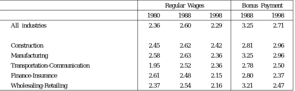
Recent issues of the Bureau of Statistics’ Family Income and Expenditure Survey (FIES ) re-ports, calculate and print elasticities of expenditure on each item with respect to total living expenditure, using broader categories (e.g., fresh meat and fish) rather than individual products of beef and pork (see Table 3 ). These elasticities are all positive, even for rice. However, it Table 2 Wage disparity by age, 1980, 1988 and 1998 ―the case of male college graduates (the ratios of 50-54 years old with 30+ years sevice/25-29 years old with 5-9 years service)
Regular Wages Bonus Payment
1980 1988 1998 1988 1998 All industries 2.36 2.60 2.29 3.25 2.71 Construction 2.45 2.62 2.42 2.81 2.96 Manufacturing 2.58 2.63 2.36 3.25 2.96 Transportation-Communication 1.95 2.52 2.36 2.78 2.50 Finance-Insurance 2.61 2.48 2.15 2.80 2.37 Wholesaling-Retailing 2.37 2.54 2.16 3.21 2.47
Source: Nakamura, A. “Analysis of Wage Statistics,” p.263, 2001.
Table 3 Estimates of elasticity of expenditure on selected food groups to living expenditure, 2000 and 2003, as reported by FIES
2000 2003
Elasticity T-value Elasticity T-value
All food 0.63 30.44 0.66 30.47
Rice 0.31 8.34 0.21 4.89
Bread 0.67 10.92 0.67 12.46
Noodles 0.41 5.87 0.48 8.93
Fresh fish and shell fish 0.54 10.52 0.51 9.53
Fresh meat 0.74 19.03 0.75 19.47 Fluid milk 0.54 12.75 0.57 15.48 Eggs 0.51 11.72 0.52 11.16 Fresh vegetables 0.50 15.20 0.46 12.32 Fresh fruit 0.41 4.60 0.31 4.44 Eating-out 1.19 14.52 1.31 16.64 Alcoholic beverage 0.43 6.48 0.56 8.30
20
is commonly accepted that the income elasticity of rice and a number of other goods, includ-ing fresh vegetables has been negative for some times. Why don’t the FIES estimates confirm this, or isn’t the common notion objectively conceived? If older Japanese, more specifically the older cohorts, consume more rice and fresh vegetables, respectively than the young (Ishi-bashi, 1997 and 2004; Mori, et al., 2004), it may be that the simple cross-sectional regression with no regard for age factors would produce positive coefficients. This is because households headed by older persons before retirement in Japan have, on average, much higher income per person than households headed by younger persons.
2. Structure of the Paper
In the following sections, we try to isolate the impact of the age factors on food consump-tion and then determine the elasticity of demand for certain foods with respect to household expenditure level, controlling for the age factors. We first use cross-section approaches, and then time-series approaches. Taking advantage of a very large sample, we move progressively from examining household consumption across subsets provided by the panel data to using cohort techniques to per capita individual consumption by age, always trying to increase our evidence about the impact of different income levels on food consumption. More specifically, in conducting cross-sectional analysis in Section 3, we classify the panel data of household food consumption by household types provided by the survey data structure, such as house-holds containing a married couple in their 30s and two children aged under 10; a married couple in their 60s with no child; etc. In conducting time series analysis (over the past 20 years) in Section 4, we first follow the traditional approaches of using per capita consumption data obtained by simple division (dividing household consumption by the number of persons within the household) to look at income effects. Next, we derive individual consumption by age, incorporating household composition matrices by household head. By applying a Bayesian cohort model to the time-series consumption data organized by age, we determine “pure time effects” in consumption changes since the early 1980s that are independent of both age and cohort effects. In Section 5 we compare the estimates obtained from both cross-sectional and time-series approaches, with and without controlling for age, and discuss the plausibility of the signs and magnitudes of income elasticities that we derive for selected products.
Age-Free Income Elasticities of Demand for Foods: New Evidence from Japan
21
In this article, we focus on income effects for a broader set of commodities. Several technical refinements, though minor in nature, were undertaken in deriving per capita individual con-sumption from the household data and also in decomposing individual concon-sumption into age, period, and cohort effects.
To summarize, these are the steps taken to analyze income effects on consumption:
1. Regress consumption per person against household income per person in each year of the sample (cross-section)
2. Regress consumption per household against household income for households of simi-lar age and structure in each year of the sample (cross-section)
3. Regress average consumption per person against household expenditure (as proxy for income) per person over the years of the sample (annual time-series)
4. Derive individual consumption by age, using family composition matrices from the panel data
5. Decompose changes in consumption per person into age, cohort, and time effects 6. Regress grand mean plus time effects against average household expenditure per person
over the years of the sample (annual time-series)
3. Analysis of Panel Data
a. Data sourcesThe Bureau of Statistics of the Government of Japan has conducted year-round surveys of household purchases of various goods and services, including housing and education, since the late 1940s. Approximately 8,000 chosen urban households across the country, excluding single person households1, are requested to keep daily accounts of all transactions, both in money
and kind (the books are collected monthly) over a six month period. One sixth of the house-holds are replaced each month. The Bureau publishes the compiled results in monthly and an-nual reports on the (Family Income and Expenditure Survey) FIES .
22
in 2002 (MAFF, 2004). It is likely that most fresh fruit, except for some minor varieties for confectionaries, is consumed at home.
The panel data survey approximately 8,000 households for 12 months, or 96,000 households each year. In practice, it is impossible to follow an individual household’s reports across the 6 months in which it is in the survey. As noted above, one sixth of the households are ro-tated in/out each month. We treat each month’s data as essentially independent from those of the other months. Since none of the products selected for our analysis exhibits distinct sea-sonality, we analyze 12 months of data, approximately 96,000 households each year, in the following investigations.
In filling out the questionnaire, each household is requested to report annual income by all members of the household earned during the past 12 months, which does not include imputed income to owned housing and use of personal savings.2 Monthly household purchases are
re-gressed against income for the preceding year (not for the particular month).
Apparent “outliers” in monthly purchases are problematic. For example, one household pur-chased 360 kg of rice in one month, compared to the average 15.3 kg purchase for all households of the same type in that month. The monthly purchase amount of 360 kg could possibly be an error in reporting or data entry, or very likely reflect gift uses for distant friends and relatives. Fresh fruit data often reflect likely purchases of local fruits in season for shipment to friends in other cities. Beef and pork data raised few concerns. In order not to bias estimates, such outliers should be eliminated beforehand. It is not easy, however, how to delineate normal and abnormal observations in the panel data we have at our disposal. Since criteria for outliers such as Smirnov and Grubb’s tests proved not very efficient for our data3, we excluded those data with purchases more than 3 times the median of observations
within each household category. In the case of rice, we calculated the median purchase while excluding zero purchases (because a number of Japanese households purchase rice in large amounts only every two, or possibly three months, zero purchase of rice rarely implies zero consumption for rice)4.
1. In July 1999, the households engaged in agriculture, forestry and fisheries were included in the cover-age of Survey but were independently tabulated until the end of the year. In this investigation, we se-lected only urban households for analysis. In January 2002, the households of one-person were incorpo-rated into the coverage of FIES . These households had been independently surveyed by the Income and Expenditure Survey for One-person Households from 1995 through 2001.
Age-Free Income Elasticities of Demand for Foods: New Evidence from Japan
23
2000). We classify the data by the types of household first, since we have quite large number of sam-ples and partly because income as reported by FIES is not the same in content as stated in the text (the imputed rent to the residence owned and the drawings from the saving are not counted which should account for large portion of actual expenditures by those retired households in their 60s, for ex-ample.
3. Grubbs’ test detects one outlier at a time. This outlier is expunged from the data-set and the test is iterated until no outliers are detected.
4. Dong, Shonkwiler, and Capps(1998) suggest that “the appropriate treatment of non-consuming house-holds constitutes an area of research that requires careful and thoughtful analysis.” (472). Perali and Chavas (2000) state, “the behavioral information contained in the observations with zero expenditures has significant econometric as well as economic implications.” (1024). In the case of rice in Japan, however, the vast majority of households consume rice almost every day and zero expenditures on rice in particular months may simply manifest that they held sufficient stocks from purchases in the preced-ing months.
b. Basic model
For simplicity and the ease of interpretation, the following basic form is chosen: log vi = a + b log v0 ……(1)
or
log qi = a + b log v0 ……(2) where:
vi is expenditure on the particular product, qi is the quantity of the particular product pur-chased (= consumed), and v0 is income.
Following the traditional approach taken by Prais and Houthakker (1971), we first regress monthly household purchases of the individual products−rice, pork, beef, and aggregate fresh
fruit−against household incomes. Prais and Houthakker use household expenditure and
quan-tity consumed per person5 on/of a particular product against total expenditure (as proxy for
income6) per person. Our first exercise simply regresses household demand per person for the
selected four foods against household income per person in each year of our sample (i.e., a cross-section regression). Obtained results are in Tables 4-A and 4-B, and are discussed later.
24
members. Indicative results are discussed in the subsequent section 3d below.
5. Food is “almost entirely private (goods)”, the scope for economies of scale is likely to be very small (Deaton and Zaidi, 2002, 46-49).
6. In comparing household incomes of different size and composition, the problem of scale economies should be considered (Prais and Houthakker, op. cit., 146-152; Deaton and Zaidi, 2002, 46-51). In our subsequent analysis, however, the same size households are compared, by classifying the data by the type of households as mentioned in the text.
c. Cross-sectional analysis of the pooled households
Tables 4-A and 4-B show the income elasticity estimates for rice, pork, beef and fresh fruit, respectively, using the above forms (1) and (2)7, for the calendar years, 1987, 1991, and 1999.
The results in Table 4-A represent income elasticities of expenditure on the food product. Ex-penditure on a product reflects the price paid as well as the quantity purchased, and thus re-tains information about the quality, as well as quantity, of the food choice by the household. The results in Table 4-B correspond to the ordinary income elasticities of demand which re-late to the physical amount of consumption (Stigler, 1966, p. 33; Friedman, 1976, p.45), with-out considering the quality/variety elements of the product. For our products, this can be
im-Table 4-A Estimates of income elasticities of at-home expenditures for rice, fresh pork, fresh beef, and fresh fruit, using pooled household data, 1987, 1991, and 1999
Rice Fresh Pork Fresh Beef Fresh Fruit 1987 Elasticities −0.03(−1.44) 0.18(10.72) 0.35(19.38) 0.20(7.52) Adj. R2 0.04 0.82 0.94 0.69 1991 Elasticities −0.06(−1.94) 0.17(10.96) 0.29(21.08) 0.08(2.05) Adj. R2 0.10 0.83 0.95 0.11 1999 Elasticities −0.18(−4.42) 0.14(12.04) 0.18(8.10) −0.06(−1.19) Adj. R2 0.43 0.85 0.72 0.02
Table 4-B Estimates of income elasticities of at-home consumption (physical quantity) of rice, fresh pork, fresh beef, and fresh fruit, using pooled household data, 1987, 1991, and 1999
Rice Fresh Pork Fresh Beef Fresh Fruit 1987 Elasticities −0.07(−2.92) 0.10(5.29) 0.25(19.57) 0.11(4.64) Adj. R2 0.23 0.52 0.94 0.45 1991 Elasticities −0.09(−3.12) 0.11(6.03) 0.24(15.57) 0.02(0.59) Adj. R2 0.26 0.59 0.91 −0.03 1999 Elasticities −0.22(−6.02) 0.10(9.54) 0.14(7.78) −0.11(−2.31) Adj. R2 0.59 0.78 0.70 0.15
Age-Free Income Elasticities of Demand for Foods: New Evidence from Japan
25
portant. For example, in Japan wagyu beef and imported beef or sirloin and ground beef have very different prices and uses. In terms of quantity, however, this analysis is forced to treat them as the same product.
All the elasticity estimates in Tables 4-A and 4-B, except for rice and fresh fruit, carry positive signs, with the parameter estimate significantly different from zero in most cases.
7. Data is converted into per capita basis, by dividing expenditure/quantity and incomes by number of household members in this sub-section, since we are dealing with all households of different sizes.
d. Panel data classified by household types
In a first assessment of the age factors in at-home food consumption, we selected the fol-lowing four categories of household8: a married couple in their 30s and two children under
10 years of age; a married couple in their 40s and two teen-age children; a married couple in their 50s and a child in the 20s; and a married couple in their 60s with no dependents.
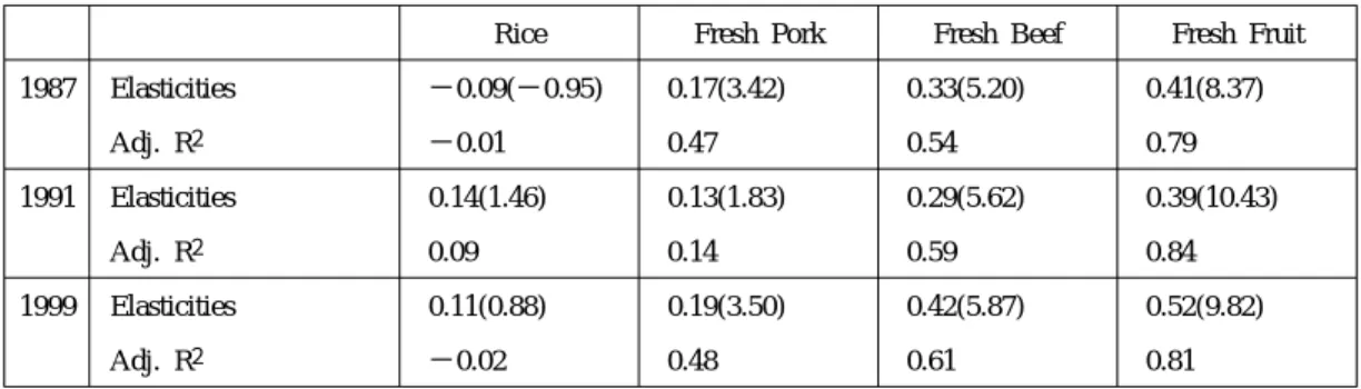
Tables 5-A and 5-B show the regression results by household type: elasticities of expendi-ture and of quantity of individual consumption with respect to annual income, for the same period as for Tables 4-A and 4-B. Notable differences between Tables 4-A&B and 5-A&B in-clude:
・(1) the elasticities for fresh fruit in Tables 5-A and 5-B are positive in sign, with good
sta-tistical performance; and
・(2) with a few exceptions, elasticities for pork in Tables 5-A and 5-B are statistically not
different from zero, when the data are broken out by these household types, whereas the coefficients (for pork) carry significantly positive signs with high R2s in Tables A and 4-B when no age factors considered.
Table 5-A Estimates of income elasticities of at-home expenditures for rice, fresh pork, fresh beef, and fresh fruit, 1987, 1991,and 1999
I : HH 30s with 2 children under 10
26
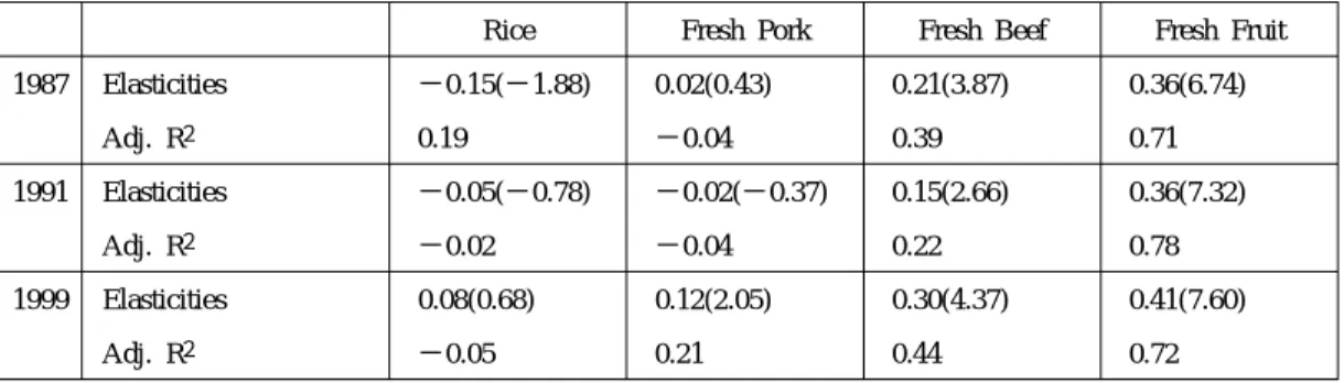
Table 5-B Estimates of income elasticities of at-home consumption (physical quantity) of rice, fresh pork, fresh beef, and fresh fruit, 1987, 1991, and 1999
I : HH 30s with 2 children under 10
Rice Fresh Pork Fresh Beef Fresh Fruit 1987 Elasticities −0.15(−1.88) 0.02(0.43) 0.21(3.87) 0.36(6.74) Adj. R2 0.19 −0.04 0.39 0.71 1991 Elasticities −0.05(−0.78) −0.02(−0.37) 0.15(2.66) 0.36(7.32) Adj. R2 −0.02 −0.04 0.22 0.78 1999 Elasticities 0.08(0.68) 0.12(2.05) 0.30(4.37) 0.41(7.60) Adj. R2 −0.05 0.21 0.44 0.72
Notes: (1) figures in parentheses denote t-values.
Table 5-A Estimates of income elasticities of at-home expenditures for rice, fresh pork, fresh beef, and fresh fruit, 1987, 1991,and 1999
II : HH 40s with 2 teenaged children
Rice Fresh Pork Fresh Beef Fresh Fruit 1987 Elasticities −0.12(−3.02) 0.15(2.56) 0.46(7.26) 0.40(7.73) Adj. R2 0.28 0.19 0.69 0.72 1991 Elasticities −0.09(−1.35) 0.18(4.08) 0.31(5.42) 0.37(8.06) Adj. R2 0.04 0.42 0.56 0.74 1999 Elasticities 0.15(0.81) 0.17(2.18) 0.21(2.24) 0.56(4.22) Adj. R2 −0.03 0.26 0.17 0.60
Table 5-B Estimates of income elasticities of at-home consumption (physical quantity) of rice, fresh pork, fresh beef, and fresh fruit, 1987, 1991, and 1999
II : HH 40s with 2 teenaged children
Rice Fresh Pork Fresh Beef Fresh Fruit 1987 Elasticities −0.19(−4.81) 0.12(1.74) 0.37(5.07) 0.30(5.40) Adj. R2 0.51 0.12 0.51 0.55 1991 Elasticities −0.17(−2.55) 0.09(2.30) 0.24(4.29) 0.32(5.77) Adj. R2 0.23 0.16 0.44 0.59 1999 Elasticities 0.04(0.27) 0.07(1.07) 0.06(0.65) 0.38(3.86) Adj. R2 −0.04 0.01 −0.03 0.56
27
Table 5-A Estimates of income elasticities of at-home expenditures for rice, fresh pork, fresh beef, and fresh fruit, 1987, 1991, and 1999
III : HH 50s with 1 child in 20s
Rice Fresh Pork Fresh Beef Fresh Fruit 1987 Elasticities −0.19(−1.68) 0.14(2.46) 0.23(3.42) 0.28(3.74) Adj. R2 0.13 0.18 0.32 0.38 1991 Elasticities −0.21(−2.96) −0.04(−0.60) 0.24(2.30) 0.18(3.13) Adj. R2 0.26 −0.03 0.16 0.21 1999 Elasticities −0.10(−0.84) 0.05(0.88) 0.07(0.72) 0.30(4.13) Adj. R2 −0.02 −0.01 −0.02 0.42
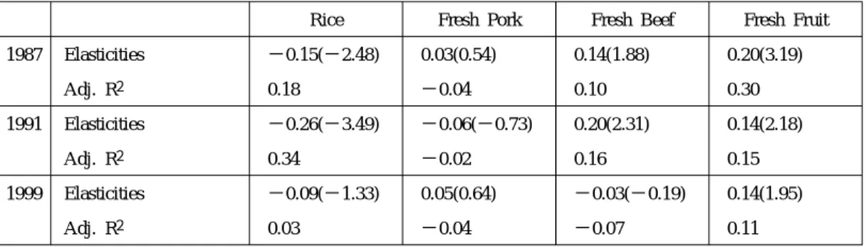
Table 5-B Estimates of income elasticities of at-home consumption (physical quantity) of rice, fresh pork, fresh beef, and fresh fruit, 1987, 1991, and 1999
III : HH 50s with 1 child in 20s
Rice Fresh Pork Fresh Beef Fresh Fruit 1987 Elasticities −0.15(−2.48) 0.03(0.54) 0.14(1.88) 0.20(3.19) Adj. R2 0.18 −0.04 0.10 0.30 1991 Elasticities −0.26(−3.49) −0.06(−0.73) 0.20(2.31) 0.14(2.18) Adj. R2 0.34 −0.02 0.16 0.15 1999 Elasticities −0.09(−1.33) 0.05(0.64) −0.03(−0.19) 0.14(1.95) Adj. R2 0.03 −0.04 −0.07 0.11
Notes: (1) figures in parentheses denote t-values.
Table 5-A Estimates of income elasticities of at-home expenditures for rice, fresh pork, fresh beef, and fresh fruit, 1987, 1991, and 1999
IV : HH 60s with no children
28
8. The nuclear family of two generations (parents and children) is the dominant form of Japanese house-holds today, accounting for 79.2 % of all househouse-holds, excluding single person-househouse-holds, in 1995 (Sta-tistics of Japan, 2000).
4. Analysis of Time-series Data
a. Changes in average per capita household consumption
Annual reports of FIES provide data pertaining to average number of persons; (total) living expenditure; expenditure, quantity, and price of individual commodities and their sub-groups purchased; and expenditure on certain individual goods and services. The Bureau of Statistics publishes consumer price indexes (CPI) for overall consumption, and by commodity group for each month and year. In the following time-series analysis, we use the expenditures and prices deflated by the overall CPI.
FIES began publishing household purchases of individual commodities and services by the
age group of the household head (HH) in 1979. We will draw upon this information in this study to estimate individual consumption (= per capita consumption by individual members of a household) by age. This is partly the reason why we cover the period from 1979 on. The decade since the early 1980s is known as the years of the economic “bubble” and the years after the bubble burst in 1991 are often called the “lost decade” (Tanaka, 2002). The stock price (TOPIX) sharply rose from 474.0 in 1980 to 997.2 in 1985, and 2177.96 in 1990 and then fell to 1178.14 in 1998 and 974.49 in 2002. Urban land prices steadily rose from 24.5 in 1980 to 33.6 in 1985 and 103.0 in 1991 and fell to 39.0 in 2000 (six largest cities: 1990 =100; Economic Annals 2002). Consumer prices, including foods, however, have stayed rela-Table 5-B Estimates of income elasticities of at-home consumption (physical quantity) of rice, fresh pork, fresh beef, and fresh fruit, 1987, 1991, and 1999
IV : HH 60s with no children
Rice Fresh Pork Fresh Beef Fresh Fruit 1987 Elasticities −0.20(−4.08) −0.08(−1.14) 0.32(5.22) 0.16(3.74) Adj. R2 0.48 0.02 0.58 0.35 1991 Elasticities −0.06(−1.10) −0.05(−1.11) 0.20(2.60) 0.32(8.38) Adj. R2 0.01 0.01 0.32 0.85 1999 Elasticities −0.10(−1.76) −0.07(1.71) 0.15(2.99) 0.23(4.06) Adj. R2 0.08 0.07 0.35 0.51
Age-Free Income Elasticities of Demand for Foods: New Evidence from Japan
29
tively stable during these turbulent years, with the overall CPI rising from 75.2 in 1980 to 92.1 in 1990 and 100 in 2000 (Appendix Table 1).
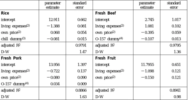
Using the data across years, we repeat with time series regressions the process used with annual cross-sections of the data. Table 6 presents the non age-compensated estimates of in-come and own price elasticities of demand for rice, pork, beef, and fresh fruit, obtained from ordinary double log LS method−see equation (3), regressing per capita consumption of an
in-dividual commodity (CapQ ) against real per capita living expenditure (RLE ) and the real price of the commodity (RP ) calculated as the average unit price paid (adjusted by the over-all CPI).
ln(CapQ ) = a + b ln(RLE ) + c ln(RP ) + D ……(3)
The regressions use the data from the past two decades since 1980. The time period cov-ered excludes 1979, the year of the second oil crisis in Japan when all the economic activi-ties were disturbed by the sudden hikes in the crude oil prices from $13.89 per barrel in 1978 to $23.08 in 1979 and $36.94 in 1980. The year 2001 is omitted for beef and pork, because of the incidence of BSE in the domestic beef production in that year which caused demand for beef to be quite unstable and demand for pork to surge upward.
Japanese rice production suffered from a devastatingly cool summer in 1994, and the result-ing influx of imported rice (gaimai) was said to have diverted Japanese consumers’ taste to other staples, such as spaghetti, Chinese noodles, and the like. For that reason, a “chill” dummy variable is applied to the years 1994 through 2001(with a zero value for 1980-93, and a value of 1 for 1994-2001)9. In the case of beef and pork, the incidence of E-coli
O-157 in 1996 seems to have had lasting impacts on household consumption of the red meats. The dummy variable, O-157 was applied to the time series regression for both beef and pork throughout in this study10, including for the age factor-controlled analysis.
30
As early as the mid-1980s, a few market experts noticed that young Japanese were con-suming less fresh fruit (Endo, 1986). The 1994 White Paper on Agriculture drew public atten-tion to the phenomenon of “wakamono no kudamono-banare” (leaving off fresh fruit by the young), by analyzing the time-series consumption of mandarins and apples using data organ-ized by the age group of the household head (MAFF, 1995). In order to investigate if declin-ing overall fresh fruit consumption over time, and changes in the consumption of the other foods, are a function of rising incomes or changing tastes by population segments in an aging society, or both, we incorporate age factors into the time-series analysis of food consumption in the subsequent sections.
9. A chill dummy was first applied to the year 1994, resulting in better statistical performance, and then to 1995, 1995 and 1996, and so on in turn to conclude that demand for rice seems to have been ad-versely affected since 1994, i.e., the demand curve has been shifted leftward that much since then. 10. An O-157 dummy was first applied to the year 1996 only, then to subsequent years in turn to
con-clude that demand for beef may have been adversely affected since 1996 on. On the other hand, the demand for pork seems to have been positively affected to some extent.
Table 6 Elasticities of demand for rice, fresh pork, fresh beef, and fresh fruit: simple per capita con-sumption as dependent variable, using OLS double log form for the period of 1981 to 2001(1)
parameter estimate standard error parameter estimate standard error
Rice Fresh Beef
intercept 12.911 0.662 intercept 2.745 1.017
living expenses(2) −1.388 0.081 living expenses(2) 1.081 0.102 own price(2) 0.068 0.054 own price(2) −0.395 0.059 chill dummy(3) −0.081 0.015 O-157 dummy(4) −0.107 0.013
adjusted R2 0.9791 adjusted R2 0.9795
D-W 1.47 D-W 1.36
Fresh Pork Fresh Fruit
intercept 13.956 1.397 intercept 11.7955 0.651
living expenses(2) −0.722 0.137 living expenses(2) −1.098 0.121 own price(2) −0.080 0.090 own price(2) −0.150 0.121 O-157 dummy(4) 0.034 0.009
adjusted R2 0.8866 adjusted R2 0.8941
D-W 1.63 D-W 0.98
Age-Free Income Elasticities of Demand for Foods: New Evidence from Japan
31
b. Deriving individual consumption by age from household data classified by the age groups of household head
FIES has published household consumption by the age group of the household head (HH)
in its annual reports since 1979. It has been common for analysts to use the HH data di-vided by the number of persons in respective households as proxies to derive estimates of consumption per person by respective age groups (Yamaguchi, 1987; Saito, 1993; Matsuda and Nakamura, 1993; MAFF, 1995). In view of the fact that the prevalent households of size 4 usually comprise two adults--a HH and his spouse and two children, or three adults--the HH, his spouse and his mother or father and one child, the simple division approach involves in-herent shortcomings. Consumption by non-adults is not available (all HHs are adults) and even the estimates for the HH age groups could be biased by ignoring other family members of different ages, their children and parents who live with them.
Using the family composition matrices from the panel data, we determine individual con-sumption by all members of household by age in a much more realistic way, by using the Mori and Inaba model (1997), modified by Tanaka, Mori, and Inaba (2004), which is pre-sented below.
In addition to 10 equations representing household consumption by 10 HH age groups, equation (4), we have 14 sub-equations representing the side-constraints of zenshinteki henka (gradual changes between successive individual age groups), equation (5):
!
%#" "%
!%&$%!#&#"& (j = 1 to 10; i = 1 to 15)……(4)
"!!$'!"!!$'""#"' (k = 1 to 14)……(5)
where:
Xi = average consumption by subject in the ith age group, from the youngest, 1-9, to 10-14,
……, 70-74, and 75+, the oldest;
Cij = family composition: number of persons in the ith age group in the jth HH age group;
Hj = average household purchase by the jth HH age group;
E = error term.
We estimate parameters, Xi, using WLS (weighted least squares) to minimize
! &#" "! (&"&#"! '#" "$ ('"'# ……(6)
with (&and (' set at 1.0 to start, and then modified according to standardized residuals
3
2
3
3
3
4
3
5
36
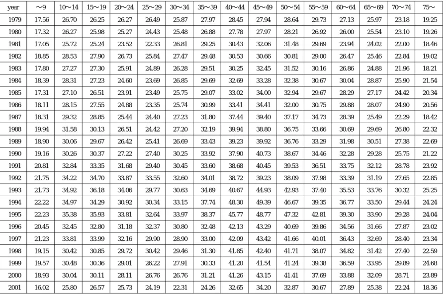
Tables 7, 8, 9, and 10 show our estimates of per capita individual consumption by age of rice, pork, beef, and fresh fruit, respectively from 1979 to 2001. More detail about changes and trends in food consumption by age groups is available in earlier publications (Mori and Inaba, 1997; Lewis, Mori and Gorman, 2001; Mori, Clason, Dyck, and Gorman, 2001). It is clear that changes in individual consumption in the past two decades vary both in patterns and magnitude by age. For example,
! rice consumption decreased appreciably across all ages, but non-adults and young
adults in their 20s and 30s show much sharper declines than the older adults in their 60s and 70s;
! non-adults and young adults in their 20s and 30s decreased their pork
consump-tion around 20%, whereas older adults in their 60s and 70s increased it nearly 10%;
! beef increased across all age groups but the increase is the greatest among those
in their 40s and 50s;
! and, most strikingly, fresh fruit declined more than 50% among non-adults and
young adults in their 20s and 30s, whereas the older age groups 65 years old and above increased their consumption slightly over the same period.
Those individuals who were in their 50s in 1980 have aged to their 70s in 2000, and, likewise, those in their 20s and 30s in 1980 were in their 40s and 50s in 2000, likely retain-ing the eatretain-ing habits acquired when they came of age 20 to 30 years ago.11 To incorporate this information, we need to introduce a new analytical perspective: generation, or birth co-hort.
11. One’s eating habits may be formed firmly, independently from parental influence, during one’s adoles-cence (refer to section 3, Chapter 8, Mori, eds., 2001).
c. Decomposing changes in per capita individual consumption into age, cohort, and (pure) time effects
By the simple A/P/C (age/period/cohort) model of cohort analysis, per capita individual con-sumption by subject, i years old in the year, t, Xit is expressed as follows:
%')""!!'!$)!#(!&') ……(7)
where:
B = grand mean effect;
Ai = age effect to be attributed to age i years old;
Pt = period effect to be attributed to the year t;
Age-Free Income Elasticities of Demand for Foods: New Evidence from Japan
37 eit = random error.
Our basic cohort tables consist of 23 rows, from 1979 to 2001, and 14 columns, from age group of 10-14 to 75+, and reflect the assumption that one’s eating habits are formed during one’s young adolescent years, or 12 columns, from 20-24 to 75+, if we assume that one’s eating habits are formed only during one’s young adulthood, independently from parental in-fluence. The oldest cohorts are those above 74 years of age in 1979, and the youngest, or the newest ones are those who are 10-14 in 2001 (if we assume the family-influenced eating habits), or who are 20-24 in 2001 (if we assume the young adult period is most formative for food tastes). Thus, we have 19 or 17 cohorts in total, depending on the assumption. The number of parameters to be estimated is 23 (years, 1979-2001) + 12 or 14 (age groups) +
17 or 19 (cohorts) = 52 or 56, and Tables 7 through 10 provide 23 × 12, or 23 × 14 =
276 or 322 observations, respectively for each commodity.
Given the large sample size, it may seem as if there should be sufficient degrees of free-dom for estimating cohort parameters, age effects, period effects, and cohort effects on top of grand mean effect. We face, however, the structural problem inherent in the ordinary A/P/C cohort model, i.e., the “identification problem” (Mason and Fienberg, 1985). If we take any two variables, say, the year of investigation, t, and the age group, i, then the cohort, the year when the subject was born, is automatically determined. In circumventing this technical diffi-culty, we are using the Bayesian cohort model developed by T. Nakamura (Nakamura, 1982 and 1986. For the less mathematically rigorous explanations, refer to Mori and Gorman, pp. 84-88, 1999; Mori, Clason, Dyck, and Gorman, pp. 321-324, 2001; Tanaka, Mori, Inaba, and Ishibashi, pp. 52-55, 2004; Mori and Clason, 2004, pp. 29-30).
38
Table 11 Changes in individual per capita consumption of rice from 1981 to 2001, decomposed into age, time and cohort effects(1)
Grand mean effects = 40.971 (kg/year)
Age Effects: Ai Time Effects: Pt Cohort Effects: Ck
Age groups(yrs.old) Calendar Year Years born
1979 ……(2) ∼1906 7.315 20−24 −7.424 1980 ……(2) 1907−11 7.220 25−29 −8.412 1981 6.448 1912−16 8.038 30−34 −7.129 1982 6.543 1917−21 8.768 35−39 −1.680 1983 7.044 1922−26 9.272 40−44 8.734 1984 5.253 1927−31 9.868 45−49 8.725 1985 5.836 1932−36 10.186 50−54 6.054 1986 4.787 1937−41 8.197 55−59 4.345 1987 3.032 1942−46 4.063 60−64 3.148 1988 0.808 1947−51 −1.454 65−69 2.594 1989 −0.145 1952−56 −7.153 70−74 −1.686 1990 −0.904 1957−61 −9.248 75∼ −7.270 1991 −1.221 1962−66 −8.726 1992 −1.858 1967−71 −9.142 1993 −1.198 1972−76 −10.359 1994 −4.423 1977−81 −13.422 1995 −5.060 1996 −4.648 1997 −4.935 1998 −3.858 1999 −3.802 2000 −3.367 2001 −4.331
Notes: (1) priors assigned to age, time and cohort effects in the estimation are: 1,1 and 1, respectively; (2) the years 1979 and 1980 are excluded from cohort calculation (refer to the text).
Table 12 Changes in individual per capita consumption of fresh pork from 1980 to 2000, de-composed into age, time and cohort effects(1)
Grand mean effects = 47.125 (100g/year)
Age Effects: Ai Time Effects: Pt Cohort Effects: Ck
Age groups(yrs.old) Calendar Year Years born
1979 ……(2) ∼1905 −14.199 20−24 4.137 1980 6.691 1906−10 −11.880 25−29 1.886 1981 4.216 1911−15 −9.869 30−34 −1.362 1982 3.978 1916−20 −6.782 35−39 −0.490 1983 2.284 1921−25 −4.604 40−44 5.094 1984 0.417 1926−30 −0.395 45−49 6.366 1985 −0.669 1931−35 2.825 50−54 3.344 1986 −0.049 1936−40 5.500 55−59 −0.448 1987 0.460 1941−45 8.568 60−64 −2.206 1988 −1.334 1946−50 8.123 65−69 −3.041 1989 −1.723 1951−55 5.822 70−74 −4.849 1990 −0.319 1956−60 2.749 75∼ −8.431 1991 −1.984 1961−65 3.843 1992 −2.162 1966−70 2.866 1993 −1.720 1971−75 3.760 1994 −2.403 1976−80 1.836 1995 −3.026 1996 −1.981 1997 −1.597 1998 −1.114 1999 0.438 2000 1.597 2001 ……(2)
39
Table 13 Changes in individual per capita consumption of fresh beef from 1980 to 2000, de-composed into age, time and cohort effects(1)
Grand mean effects = 31.215 (100g/year)
Age Effects: Ai Time Effects: Pt Cohort Effects: Ck
Age groups(yrs.old) Calendar Year Years born
1979 ……(2) ∼1905 1.071 20−24 −3.161 1980 −5.785 1906−10 −0.115 25−29 −5.035 1981 −4.957 1911−15 −1.277 30−34 −4.388 1982 −4.180 1916−20 −2.704 35−39 −1.469 1983 −4.240 1921−25 −2.368 40−44 4.267 1984 −3.016 1926−30 −2.348 45−49 6.395 1985 −3.592 1931−35 −1.614 50−54 6.250 1986 −3.054 1936−40 −0.356 55−59 4.745 1987 −1.621 1941−45 2.014 60−64 2.659 1988 −0.490 1946−50 3.532 65−69 0.750 1989 −0.117 1951−55 3.298 70−74 −2.888 1990 0.437 1956−60 1.849 75∼ −8.124 1991 1.896 1961−65 0.011 1992 2.265 1966−70 0.408 1993 3.654 1971−75 0.240 1994 5.497 1976−80 −0.821 1995 6.260 1996 2.799 1997 2.905 1998 2.005 1999 1.948 2000 1.388 2001 ……(2)
Notes: (1) priors assigned to age, time and cohort effects in the estimation are: 4, 2 and 2, respectively; (2) the years 1979 and 2001 are excluded from cohort calculation (refer to the text).
Table 14 Changes in individual per capita consumption of fresh fruit from 1981 to 2001, de-composed into age, time and cohort effects(1)
Grand mean effects = 39.784 (kg/year)
Age Effects: Ai Time Effects: Pt Cohort Effects: Ck
Age groups(yrs.old) Calendar Year Years born
1979 ……(2) ∼1906 8.499 20−24 −2.579 1980 ……(2) 1907−11 11.352 25−29 −4.537 1981 −2.274 1912−16 13.799 30−34 −5.251 1982 −1.414 1917−21 15.992 35−39 −4.456 1983 1.690 1922−26 16.958 40−44 −2.578 1984 0.959 1927−31 17.362 45−49 −1.792 1985 −0.761 1932−36 15.228 50−54 −0.601 1986 −0.493 1937−41 13.096 55−59 2.772 1987 1.846 1942−46 10.294 60−64 5.053 1988 1.333 1947−51 4.343 65−69 6.407 1989 −0.986 1952−56 −1.842 70−74 5.078 1990 −0.568 1957−61 −7.782 75∼ 2.485 1991 −1.316 1962−66 −14.414 1992 −0.897 1967−71 −19.505 1993 −0.420 1972−76 −23.954 1994 1.786 1977−81 −29.713 1995 −0.857 1996 −1.321 1997 0.317 1998 −0.147 1999 0.514 2000 1.418 2001 1.591
40
d. Regressing (grand men effect + period effects) as proxies for “pure” time ef-fects against changes in price and income over time
By replacing (capQ ) in equation (3) in 4.a. by (gm + pe : grand mean effect + period ef-fects) provided by Tables 11 through 14, as shown in equation (8) below, we estimate income and price elasticities of demand for rice, pork, beef, and fresh fruit, respectively, with age-related differences removed from the dependent variable. The time periods covered for respec-tive products are basically the same as for the analysis in 4.a, equation (3).
ln (gm + pe) = a + b ln (RLE ) + c ln (RP ) + D ……(8)
Table 15 shows the results of the regressions. Generally, we have obtained reasonably good statistical fits. More importantly, the estimated elasticities seem to better conform to the
statis-Table 15 Elasticities of demand for rice, fresh pork, fresh beef, and fresh fruit: (A) simple per capita consumption as dependent variable (replica of Table 6) and
(B) grand mean plus period effects derived from cohort analysis as dependent variable, esti-mated using OLS double log form for the period of 1981 to 2001(1)
(A) dependent variable=simple per capita consumption (B) dependent variable=grand mean+period effects Rice parameter estimate standard error parameter estimate standard error
intercept 12.911 0.662 11.843 0.595 living expenses(2) −1.388 0.081 −1.134 0.073 own price(2) 0.068 0.054 −0.025 0.049 chill dummy(3) −0.081 0.015 −0.069 0.013 adjusted R2 0.9791 0.9726 D-W 1.47 1.61 Fresh pork intercept 13.956 1.397 11.419 2.156 living expenses(2) −0.722 0.137 −0.981 0.212 own price(2) −0.080 0.090 −0.139 0.139 O-157 dummy(4) 0.034 0.009 0.050 0.014 adjusted R2 0.8866 0.8416 D-W 1.63 0.96 Fresh beef intercept 2.745 1.017 −1.132 0.920 living expenses(2) 1.081 0.102 0.993 0.092 own price(2) −0.395 0.059 −0.408 0.054 O-157 dummy(4) −0.107 0.013 −0.102 0.012 adjusted R2 0.9795 0.9820 D-W 1.36 1.41 Fresh fruit intercept 11.796 0.651 3.046 0.521 living expenses(2) −1.098 0.121 0.277 0.103 own price(2) −0.150 0.121 −0.349 0.103 adjusted R2 0.8941 0.3245 D-W 0.98 2.01
Age-Free Income Elasticities of Demand for Foods: New Evidence from Japan
41
tical inference from the findings of cross-sectional analysis in section 3, particularly in the case of fresh fruit, compared to the results from the non age-compensated time-series analysis in 4.a. The non age-compensated analysis gave rise to negative income elasticity as large as -1.10 for fresh fruit, whereas the (gm + pe) approach produced a positive elasticity, +0.28, with reasonable value close to 3, along with acceptable own price elasticity of -0.35 with t-value larger than 3 (but with lower explanatory power for the equation―R2 drops from .89 to .32).
On the other hand, the income elasticity for pork is estimated at -0.72 by the non compensated approach, compared to -0.98 by the (gm + pe) approach. For rice, the non age-age compensated estimate is -1.40 vs.-1.13 from the age-age compensated method. For beef, the elasticity estimate is 1.08 without compensation for the age-related effects, vs. 0.99, when age -related effects are separated. Except for the case of fresh fruit, we are not in the position to instantly affirm that our attempt to compensate for the age factors has produced better results than the ordinary age-neglected approach in 4.a.
5. The Impact of Age Factors in Determining Income Elasticities of Demand:
Discussion
Cross-section evidence for the quantity consumed per person indicates that rice is an infe-rior good in the sense that consumption tends to decline as income increases. Pork quantity consumed appears to be income-neutral. Beef and fresh fruit appear to be normal goods, since the quantity consumed tends to respond positively to income in present day Japan. When the age-factors are controlled, income elasticities obtained from cross-sectional panel data for se-lected years in the 1980s and 1990s seem to confirm this (see Table 5 A). When expenditure as opposed to just quantity consumed are measured, rice is found still slightly negative, and pork slightly positive with respect to income changes. In view of the fact that beef and fresh fruits vary very widely in price on the market in Japan (Mori and Lin, 1994, Chapter 1), consumers are revealed in the cross-sectional analysis to purchase the higher priced products as their income increases (Figures 1 and 2 for the cases of rice and beef, for example). As expected, the income elasticities of expenditure (on individual commodity) are generally larger than those of quantity (see Prais and Houthakker, Chapter 8 for the cases in British and Dutch households). These findings conform to our intuitions based on every day observations.
42
Fig1. Price paid for rice by annual income level of selected household types.
1987 5000 5500 6000 6500 200 400 600 800 1000 1200 Annual income(ten thousand Yen) Price paid (Yen/10kg)
1999 4000 4500 5000 5500 200 400 600 800 1000 1200 Annual income(ten thousand Yen) Price paid (Yen/10kg)
HH 40s with 2 teenaged children HH 50s with 1 child in 20s HH 60s with no children HH 40s with 2 teenaged children
HH 50s with 1 child in 20s HH 60s with no children 1987 300 200 400 500 600 200 100 300 400 500 200 400 600 800 1000 1200 Annual income(ten thousand Yen) Price paid (Yen/100g)
1999
200 400 600 800 1000 1200 Annual income(ten thousand Yen) Price paid (Yen/100g)
HH 40s with 2 teenaged children HH 50s with 1 child in 20s HH 60s with no children HH 40s with 2 teenaged children
HH 50s with 1 child in 20s HH 60s with no children
Fig1. Price paid for fresh beef by annual income level of selected household types. consumption per person has increased steadily for the past decades until recently (the inci-dence of e-coli O-157 in 1996 and that of BSE in 2001 curbed beef demand).
When the age factors, the impacts of aging and cohort-replacement as well, are eliminated from the time-series data, fresh fruit is found positively related to income changes over time, with the expenditure elasticity estimated at 0.28, compared to -1.10 without the age factor compensation. In the case of rice, an upward impact of aging seems to have been more than offset by the opposing effect of the cohort replacement, resulting in an expenditure elasticity -1.13, much lower than -1.39 estimated without age factor modifications. This may imply that an increase in income might lead to somewhat slower decreases in rice consumption in future years than anticipated from the non-age compensated econometric approaches.
Age-Free Income Elasticities of Demand for Foods: New Evidence from Japan
43
analysis, pork is found to be income-neutral, when the age factors are controlled. This gap between cross-sectional and time-series results with respect to income responses should be in-vestigated by further research.
Similar reasoning seems to apply in the case of fresh beef. The income elasticity of beef is estimated at 0.99 when age factors are considered, compared to 1.08 in the non-age compen-sated model. Examining the over-time changes in per capita individual consumption by age shown in Table 9 and the estimated cohort parameters in Table 13, the impact of both aging and cohort-replacement may have slightly accelerated overall beef consumption in the past two decades or so.
6. Conclusion
Earlier work has used the age structure and cohort composition of the Japanese population to project overall consumption of selected food products in future years, with no regard to economic impacts, i.e., changes in income and prices (Tanaka and Mori, 2004; Tanaka, Mori, Inaba, and Ishibashi, 2004; Mori and Clason, 2004). Now that we have obtained the estimates of the age-free economic parameters, the income and price elasticities determined here allow future food demand to be projected using both economic and demographic perspectives. Inte-grating the age-related factors into the demand systems approach which is the norm today (Theil, 1980; Deaton and Muellbauer,1980; Matsuda, 2000; Seal, Regmi, and Bernstein, 2003; Thompson, 2004; Gardes, Duncan, Gaubert, Gurgand, and Starzec, 2005; Reed, Levedahl, and Hallahan, 2005; Meyerhoefer, Ranney, and Sahn, 2005) remains to be done in both cross-sectional and time-series approaches.
We have demonstrated that the demographic factors such as age and generational cohorts exercise substantial influences on individual food intakes in present day Japan. As clearly shown by the differences in income elasticities, estimates of income effects can be confounded with age-related effects. Age-related influence may be unique to Japan, but, more likely, are prevalent to one degree or another in other populations, both in developed and developing countries like China and Thailand12. More research efforts should be focused explicitly on demographic aspects of food consumption, first in data collection and then the development of workable analytical techniques, using even limited information available (various LSMS work-ing papers; Trivedi, 1987; Deaton, 1987).
44
References
Blundell, R., P. Pashardes, and G. Weber. 1993. “What Do We Know about Consumer Demand Patterns from Micro Data?” American Economic Review, 83(3), June, 570-597.
Chino, Jinjiro. 2005. “Keizai Hatten nitomonau Kome Shouhikouzou no Henka (Changes in Rice Consumption Structure Accompanying Economic Development), Rice Economy in the
Interna-tional Setting, eds. by Shimizu, Kobayashi and Kaneda, Tokyo, Tokyo University of Agriculture
Press.
Deaton, A. and J. Muellbauer. 1980. Economics and Consumer Behavior, Cambridge, UK, Cam-bridge University Press.
Deaton, Angus. 1987. “Estimation of Own- and Cross-Price Elasiticies from Household Survey Data,” Journal of Econometrics, 36, Sept-Oct, 7-30.
Deaton, Angus. 1998. “Quality, Quantity, and Spatial Variation of Price,” American Economic
Re-view, 78(3), June, 418-430.
Deaton, A. and C. Paxson. 1998. “Economies of Scale, Household Size, and the Demand for Food,” Journal of Political Economy, 106(5), 897-930.
Appendix Table 1 Consumer price indices, aggregate, and food: rice, fresh meat, and fresh fruit, 1975 to 2004
Year Aggregate Food Rice Fresh Meat Fresh Fruit
1975 54.5 59.1 64.1 80.1 56.9 1976 59.7 64.4 73.7 89.6 61.1 1977 64.5 68.7 81.0 88.9 69.1 1978 67.3 71.1 85.7 88.2 68.7 1979 69.8 72.6 87.6 87.3 71.0 1980 75.2 77.0 90.1 88.7 71.9 1981 78.8 81.1 93.2 92.4 80.4 1982 81.1 82.6 96.7 93.5 77.6 1983 82.5 84.3 99.0 95.0 77.3 1984 84.4 86.6 102.7 95.2 82.5 1985 86.1 88.1 106.0 94.6 92.1 1986 86.7 88.3 106.8 93.3 85.1 1987 86.7 87.5 106.8 91.3 80.5 1988 87.3 88.1 105.0 90.3 81.5 1989 89.3 90.1 106.6 91.5 89.1 1990 92.1 93.7 107.8 93.7 99.7 1991 95.1 98.2 107.7 96.3 110.9 1992 96.7 98.7 111.6 97.7 112.2 1993 98.0 99.8 114.7 97.1 99.0 1994 98.6 100.6 125.6 95.9 104.0 1995 98.5 99.4 110.7 95.9 107.6 1996 98.6 99.3 108.0 97.1 107.5 1997 100.4 101.1 107.1 101.3 104.8 1998 101.0 102.5 102.8 102.4 105.3 1999 100.7 102.0 104.4 101.6 108.5 2000 100.0 100.0 100.0 100.0 100.0 2001 99.3 99.4 96.9 99.7 99.2 2002 98.4 98.6 96.5 100.4 95.8 2003 98.1 98.4 100.1 101.7 96.6 2004 98.1 99.3 109.1 105.6 100.3
Age-Free Income Elasticities of Demand for Foods: New Evidence from Japan
45
Deaton, A. and S. Zaidi. 2002. Guidelines for Constructing Consumption Aggregates for Welfare
Analysis, Living Standards Measurement Study (LSMS) Working Paper No. 135, Washington, D.
C., The World Bank.
Dong, D., J.S. Shonkwiler, and O. Capps, Jr. 1998. ”Estimation of Demand Functions Using Cross
-Sectional Household Data: The Problem Revisited,” American Journal of Agricultural Economics, 80 (August), 466-73.
Endo, Hajime. 1986. Executive Director, Japan Federation of Horticultural Cooperative Associations, Personal Communications on various occasions.
Friedman, Milton. 1976. Price Theory, Chicago, Aldine Publishing Company.
Gardes, F., S.Langlois, and D.Richaudeau. 1996. “Cross-section versus time-series income elastici-ties of Candadian consumption,” Economic Letters, 51, 169-175.
Gardes, F., G.D.Duncan, P.Gaubert, M.Gurgand, and C. Starzec. 2005. “Panel and Pseudo-Panel Es-timation of Cross-Section and Time Series Elasticities of Food Consumption: The Case of U.S. and Polish Data,” Journal of Business and Economic Statistics, 23(2), April, 242-253.
Han, Doo Bong. 2005. “Dilemmas and Challenges of Korean Rice Economy after the Rice Nego-tiation,” in Proceedings for Workshop on Rice in the World at Stake, March 13-14, Tokyo,39-53. Ishibashi, Kimiko. 1997. “Demand Forecast and Trends in Vegetable Consumption,” Japanese
Jour-nal of Farm Management, Vol. 35, 32-41 (in Japanese).
Ishibashi, Kimiko. 2004. “Changes in Household Rice Consumption by the Household Type and Income Level,” Journal of Food System Research, Vol. 11, 1-15 (in Japanese).
Isvilanonda, Somporn. 2005. “Trend in Rice Consumption in Thailand,” in Rice in the World at
Stake, op. cit., 55-65.
Ito, S., E. Wesley., F. Peterson, and W.R.Grant.1989. “Rice in Asia: Is It Becoming Inferior Good?” American Journal of Agricultural Economics, 71(1), February, 32-42.
Japanese Government, Bureau of Statistics, Family Income and Expenditure Survey, Annual Report, various issues, Tokyo.
Japanese Government, Bureau of Statistics, FIES, Panel Data, various months, Courtesy: Bureau of Statistics through Ministry of Agriculture, Forestry and Fisheries.
Japanese Government, Agency for General Affaires. 2000. Statistics of Japan, Tokyo.
Japanese Government, Ministry of Agriculture, Forestry and Fisheries. 1995. White Paper on
Agriculture-1994, Tokyo.
Japanese Government, MAFF. 2004, Personal Communications
Japanese Government, Prime Minister’s Office, Economic and Social Research Institute, Economic
Annals 2002, Tokyo.
Kooreman, P. and S. Wunderink. 1997. The Economics of Household Behavior, New York, St. Martin’s Press.
Lewis Hendrickson, M., H. Mori, and Wm. D. Gorman. 2001. “Estimating Japanese At-home Food Consumption by Age Groups while Controlling for Income Effects,” Cohort Analysis of Japanese
Food Consumption, eds. by H. Mori, 93-121.
Magota, Ryouhei. 1997. “Wages and Lifetime Livelihood Guarantee,” in Today’s Wage Problems, eds. by Social Policy Editorial Committee, Kyoto, Keibunsha (in Japanese).
Mason, T. and S.E. Fienberg. 1985. Cohort Analysis in Social Research: Beyond the Identification
Problem. New York. Springer-Verlag.
Matsuda, Toshinobu. 2004. “Incorporating Generalized Marginal Budget Shares in a Mixed Demand System,” American Journal of Agricultural Economics, 86(4) November, 1117-1126.
46
Classified by Age of a Household,” Journal of Rural Economics, Vol. 64, 213-220 (in Japanese). Meyerhoefer,C., C. Ranney, and D. Sahn. 2005. “Consistent Estimation of Censored Demand
Sys-tems Using Panel Data,” American Journal of Agricultural Economics, 87(3), August, 660-672. Minotani, Chiohiko. 1992. Robust Estimation in Econometrics, Tokyo, Chiga-shuppan (in Japanese). Mori, Hiroshi (eds.). 2001. Cohort Analysis of Japanese Food Consumption―New and Old
genera-tions, Tokyo, Senshu University Press.
Mori, H. and B.H. Lin. 1994. Japanese Beef Market―Distinctly Unique, Tokyo, Senshu University
Press.
Mori, H. and T. Inaba. 1997. “Estimating Individual Fresh Fruit Consumption by Age from House-hold Data, 1979 to 1994,” Journal of Rural Economics, Vol. 69(3), 175-85.
Mori, H. and Wm. D. Gorman. 1999. “A Cohort Analysis of Japanese Food Consumption: Old and New Generations,” Senshu University Economic Bulletin, Vol. 34(2), 71-111.
Mori, H., D.L. Clason, J. Dyck, and Wm. D. Gorman. 2001. “Age in Food Demand Analysis―A Case Study of Japanese Household Data by Cohort Approach,” Cohort Analysis of Japanese
Food Consumption, eds. by H. Mori, 311―345.
Mori, H., M. Tanaka, and T. Inaba. 2004. “Predicting At-home Consumption of Rice and Fresh Fish under a Rapidly Aging: A Cohort Approach,” The Annual Bulletin of Social Science, Vol. 38, Senshu University, 41-62 (in Japanese)..
Mori, H. and D.L. Clason. 2004. “Cohort Approach as an Effective Means for Forecasting Con-sumption in an Aging Society: The Case of Fresh Fruit in Japan,” Senshu University Economic
Bulletin, Vol. 38(2), 45-70.
Mori, H. and D.L. Clason. 2004. “A Cohort Approach for Predicting Future Eating Habits: the Case of At-home Consumption of Fresh Fish and Meat in an Aging Japanese Society,”
Interna-tional Review of Food and Agribusiness Management Review, Vol. 7(1), 22-41.
Mori, H., K. Ishibashi, M. Tanaka, and T. Inaba. 2005. “Determining Income and Price Elasticities of Demand in the Presence of Age-Cohort Effects,” The Annual Bulletin of Social Science, Vol. 39, Senshu University, 39-59 (in Japanese).
Mori, H., D. Clason, and J. Lillywhite. 2006. “Estimating Price and Income Elasticities in the Presence of Age-Cohart Effects,” Agribusiness: An International Journal, 22(2), J. Wiley & Sons. Morishima, Masaru. 1984. “Shokuryou Jyuyou no Douko”(Trend in Food Demand), Journal of
Ru-ral Economics, Vol. 56(2), 63-69 (in Japanese).
Nakamura, Atsushi. 2001. “Analysis of Wage Statistics,” in Wages in Japan during the Post War
Eras, Tokyo, Social and Economic Productivity Center (in Japanese).
Nakamura, Takashi. 1986. “Bayesian Cohort Models for General Cohort Tables,” Annals of the
In-stitute of Statistical Mathematics, Vol. 38, 353-370, Tokyo.
Perali, F. and J-P Chavas. 2000. “Estimation of Censored Demand Equations from Large Cross
-Section Data,” America Journal of Agricultural Economics, 82(4), November, 1022-1037.
Prais, S.J. and H.S. Houthakker. 1971. The Analysis of Family Budgets, Cambridge at The Univer-sity Press.
Reed, A., J. Levedahl, and C. Hallhan. 2005. “The Generalized Composite Commodity Theorem and Food Demand Estimation,” American Journal of Agricultural Economics, 87(1), February, 28
-37.
Saito, Akio. 1993. “Kudamono no Keizai Bunseki (1): Nenrei to Kudamono Jyuyou”(Economic Analysis of Fruit: Age and Fruit Demand), Chuo Kajitsu Kikin Report, No. 44, Tokyo, Cuou Kajitsu Fund, 21-29.
Age-Free Income Elasticities of Demand for Foods: New Evidence from Japan
47
United States Department of Agriculture, Economic Research Service, Technical Bulletin No. 1904.
Stigler, George J. 1966. The Theory of Price, third edition, New York, Macmillan Publishing Com-pany.
Tanaka, M., H. Mori, T. Inaba, and K. Ishibashi. 2004. “Projecting Future Household Consumption of Sake and Beer―A Cohort Analysis,” Japanese Journal of Research on Household Economics,
No. 61, Winter, 50-61 (in Japanese)..
Tanaka, M., H. Mori, and T. Inaba. 2004. “Re-estimating per Capita Individual Consumption by Age from Household Data,” The Japanese Journal of Rural Economics, Vol. 6, 20-30.
Tanaka, Takayuki. 2002. Japanese Economy in the Bubble and Post-Bubble Eras, Tokyo, Nihon
-Hyouronsha (in Japanese).
Thompson, Wyatt. 2004. “Using Elasticities from an Almost Ideal Demand System? Watch out for Group Expenditure!” America Journal of Agricultural Economics, 86(4), November, 1108-1116. Theil, Henri. 1980. The System-Wide Approach to Microeconomics, Chicago, The University of
Chicago Press.
Trivedi, Pravin K. 1987. “Editor’s Introduction,” Journal of Econometrics, 36 (1987), 1-6.
Wold, Herman, in Association with L. Jureen. 1982. Demand Analysis : A Study in Econometrics, reprinted, Westport, Connecticut, Greenwood Press.
Yamaguchi, Kikuo. 1987. Changing Trends in Food Consumption, Tokyo, Nihon Keizai Shinbun
-sha (in Japanese).