楕円型固有値問題に対する精度保証付き数値計算と その応用

Kyushu University Institutional Repository

楕円型固有値問題に対する精度保証付き数値計算と その応用

長藤, かおり

Graduate School of Mathematics, Kyushu University

https://doi.org/10.11501/3150928

出版情報：Kyushu University, 1998, 博士（数理学）, 課程博士 バージョン：

権利関係：

0

Verified numerical computation for elliptic eigenvalue problems and its applications

by Kaori N agatou

Contents

1 Introduction

2 Enclosing method for eigenvalues with uniqueness property 2.1 Proble1n and the fixed point formulation

2.2 Verification conditions . ^{. . . .} . . . 2.3 Algorithm in a co1nputer . . . . 2.4 Uniqueness of the enclosed eigenvalue

3 Excluding method for eigenvalues 3.1 Motivation . . . .

3.2 Verification conditions ^. 3.3 Algorithm in a computer

4 Applications to nonlinear elliptic problems

4.1 Statement of the proble1n and the fixed point formulation . 4.2 Verification conditions . ^. . . ^. . . . ^.

4.3 Estimation of constants and algorithm 5 Numerical examples

6 Conclusions Appendix References

1

2 2 5 9 15

23 23 24 26

31 31 34 35 38 46 47 51

and its applications

Kaori N agatou

Graduate School of Mathematics, Kyushu University Fukuoka

812-8581,

Japan

1 Introduction

Several numerical methods have been proposed to verify the exact eigenvalues for infi­

nite dimensional eigenvalue problems, and in particular the eigenvalues of elliptic operators

( cf.[2],[15, 16]).

In

[2],

the method is presented to find the upper and lower bounds for eigen­

values by using some test functions, the Rayleigh-Ritz method and the Temple quotient. In

[15, 16],

given problems are connected with a simple problem, whose explicit eigenvalues are known, by using homotopy method. In this paper, we give a technique that is different from these method. This method is based on the verification method appearing in

[25],

which is a realization,including uniqueness,of the method studied in

[9-14]

applicable to nonlinear elliptic boundary value problems.

In Section

2

we apply the numerical method described in

[25]

to our eigenvalue problems.

Using this 1nethod we can confinn local uniqueness of

eigenpairs (i.e.

pairs of eigenvalues and corresponding eigenfunctions) in a certain set. In the last part of that section, we also confirm the local uniqueness separately of eigenvalues and eigenfunctions as well as the simplicity of the eigenvalues.

In section 3 we describe a n1ethod to exclude eigenvalues in order to obtain some informations about index. By this method we can separate the simple eigenvalues and we can also obtain the bound for the Eigenvalue with Smallest Absolute Value

(

ESAV

)

. This bound plays an important role for rigorous esti1nates of the nonn of the linearized operator of some nonlinear differential equations, which is described in Section

4

in detail.

In Section

5

several nu1nerical exan1ples are presented.

2 Enclosing method for eigenvalues with uniqueness property

In this section, we consider a nun1erical technique to verify the exact eigenvalues and eigen­

functions of second-order elliptic operators in son1e neighborhood of their approximations.

This technique is based on

[25]

using the l(rawczyk-like operator and the error estin1ates for the C0 finite element solution. We nun1erically construct a set containing solutions which satisfies the hypothesis of Banach's fixed point theorem for con1pact n1ap on a certain Sobolev space.

2.1 Problem and the fixed point formulation

In what follows, let

n

be a bounded convex domain in R2 and for some integer ^m, let

Hm(n)

denote the L2-Sobolev space of order ^m on

n.

Then, define

HJ(n) = { v

^E

H1(n) I v

⁼

0

^on

an}

with the inner product< ^'U,V

>Hl= (\7u, \7v)L2

for ^{'U,V E}

HJ(n),

and the norm

lluiiHl - IIVull£2

for ^{'U E}

HJ(D.),

where

(·, ·)£2

0 and

II· 11£2

represent the inner product and

0

the norm on L2

(D)

, respectively.

Now, let Sh be a finite dimensional subspace of

HJ(D)

that depends on

h (0

^<

h

^<

1).

Usually, Sh is taken to be a finite element subspace with n1esh size

h.

Also, let Pho :

HJ(n)

^{� Sh} denote the H

J

-projection defined by

We now assume the following approximation property in Sh.

Assumption 1. For any

u

^E

H

2

(

0

) ⁿ HJ(O),

(2.1)

where

Here, C1 is a positiv , numerically determined constant which is independent of

h.

The following lemma is well known

[3].

following Poisson equation:

{ ^-�¢

^{= rtjJ in}

ⁿ

¢

⁼ 0 ^on ao.

(2.2)

Furthermore, there exists a positive constant C2 satisfying

(2.3)

In particular, if

fJ

is a convex polygonal domain, we can set

C2

⁼ 1

([3]).

We consider the self-adjoint eigenvalue problem

{

^{-�u + qu =}

^AU

ⁱⁿ

^n,

u

⁼ 0 on

an, (2.4)

where q E

L00(fJ).

Since we wish to enclose eigenpairs of this problem, we consider the space

HJ(n)

^x R and define the inner product ^{< ·, ·} > HJ xR ₀ and the norm

II

^·

II

^{HI xR} ₀ by

respectively, where

wi

⁼

(ui, Ai)

^E

HJ(D)

^x R

(

^{i = 1,}

2)

and

w

⁼

(

^u,

A)

^E

HJ(D)

^x R.

Moreover, let 10 and I be the identity map on

HJ(D)

and

HJ(D)

^x R, respectively.

vVe first nonnalize the problen1

(2.4)

as find

(u, A)

E

HJ(n)

^x R s.t.

(2.5)

We then define the projection ph ^:

HJ(n)

^X R ^----* sh ^X R by

Now, let Wh

⁼

(uh, �h)

E

s h

X R

be a finite element solution of (2.5); that is,

(2.6)

We used the interval library

PROFIL

to enclose this solution in very small intervals ( cf. [4) and Section 5).

Vve will verify the existence of eigenvalues and eigenfunctions for (2.5) in

a

neighborhood of ('u, :\h) satisfying

0

in n,

0

on an. (2.7)

Note that u

E

H2(n) ⁿ HJ(n), and wh

⁼

Ph(u, �h)· We then have, by (2.5) and (2.7),

(2.8)

Defining VI

⁼

u - uh, we see that VI

E

st' where st represents the orthogonal complement of Sh in HJ(n), and we can write

It is known that the

a posteriori

estimates are, in general, much better than the

a priori

estimates, provided that the higher order base functions in sh are utilized (see [24) for details). Therefore, we use

^a posteriori

estimates for VI as below.

Let S'h

C

HI(n) be a finite element subspace whose basis consists of the union of the basis on

sh and the base functions having nonzero values on the boundary an. Define fJuh

E

S'h

^X

S'h, a vector function in two din1ension, by the L2-projection of \luh

E

L2( n )

x

L2( n ) to S'h

x

S'h.

Then, define iiuh

E

L2(n) b:v iiuh

⁼ \1

· Vuh. We then obtain the following estimation ( cf. [24]):

where Co

=

CI C2. Note that in this estimation we used the L2-estimate of VI:

�ow, in order to verify solutions

(fi, -A)

of

( 2

.5

)

near

('il, :\h),

writing

_.__ �

u

⁼ u +

u , )..

⁼

)..h

+ :>.., we can rewrite

(2.8)

as

(�h

+

�- q)(u

+

fih

+ vl

)

-

(�h- q)fih,

1.

Thus using the following compact 1nap on

HJ(D.)

x R

F(U).)

=

( ^{( -�)-1{ cs:h}

⁺

^{3:- q)(U}

⁺

^uh

^{+ Vj}

⁾

^-

();h- q)Uh} '

3:

+

in ^(U

⁺

^uh

^{+ Vj}

⁾

^{2 dx -}

¹ ) ^{' (2.9)}

where

( -�)-1

is the solution operator for the Poisson equation with homogeneous boundary conditions, we have the fixed point equation

w

⁼

F(w) (2.10)

for

w

⁼

(u, �).

2.2 Verification conditions

We now make the following assun1ption.

Assumption 2. Set

p

=

(

-u1,

0)

and define

F'(p)

as the Frechet derivative ofF at

p.

Assun1e that the restriction to

sh

X R of the operator

Ph[!- F'(p)]

:

HJ(D.)

X R ----+

sh

X R has the inverse

The validity of this assumption can be numerically checked in actual computations.

�ow as in

[13, 14),

we de ·on1po e

(2.10)

into finite and infinite dimensional parts:

(2.11)

We use a Newton-like method only for the finite dimensional part, represented by the first equation in

(2.11).

First, we define the Kewton-like operator

We next define the operator

T: HJ(D.)

^{x R ----t}

HJ(D.)

^{x R} as

T(w) Nh(w) +(I- Ph)F(w).

Then

T

becomes a compact map on

HJ (D.)

x R, and the relation

w

⁼

T(w)

^<===} w =

F(w)

holds.

Now, an arbitrary element

w

^E

HJ(D.)

x R can be uniquely written as

with

M

Vh =

L Vj¢j, j=l

(2.12)

(2.13)

(2.14)

where M =dim Sh,

{¢1}�1

is a basis of Sh,

(vj ) f= 1

a real vector. For win

(2.14)

we use the following notation:

( w )i (w)M+l (w)M+2

lvi l , i

=

1, ..

. , M,

llvj_IIH1,

0

1111·

We intend to find a fixed point to

(2.10)

in a set

W,

referred to as a 'candidate set'. Given a vector

(WI, ... , WM+2)t

such that Wi >

0 (i

=

1,

^{... , M}

+ 2),

its candidate set

W

is defined by

I\ow let

T'

be the Frechet derivative ofT. By the method described below we choose two vectors

(Y1, ... , YM+2)t, li

>

0 (i

⁼

1, .. .

^{, M} +

2)

and

(Z1, ... , Zu+2)t, Zi

>

0 (i

⁼

1,

... , M +

2)

such that

(T(O))i

^<

}i, i =1, . ..

,M+

2 ,

(T'(wl)w2)i

^<

Zi, i

⁼

1,

... , M +

2,

for any

w1, w2 E

^W.

The verification condition is described in the following theorem.

Theorem 1. If a candidate set ^W defined

by {2.15)

satisfies

Yi +

zi

^<

wi ( i

⁼

1,

... , M +

2),

then there exists a fixed point ofT in

K ₌

{

v

E H 6 ( n)

x R

1 (

v

) i

::; li +

zi ( i

⁼

1, ..

. , M +

2)}.

Moreover, this fixed point is unique within the set ^W.

In order to prove this theorem, we derive two preliminary lemmas.

Defining the norm

II

^·

llw

by

llxll w- l�i�M+2 wi '

^{= max}

(x )i x E HJ(fl)

X R,

we have the following lemma.

Lemma 2. For each

x E HJ(n)

x R,

sup

IIT'(w)xllw::;

rpax

w zi llxllw·

wEW

l�t�M +2 i

Proof.

Since W includes a ball centered at

0

and

T'(w)

is linear,for

x E HJ(n)

x R,

sup

IIT'(w)xllw

⁼

llxllw

sup

II ^{T'(w) - ll xll} II

wEW wEW X W W

(2. 16) (2.17)

(2.18)

(2.19)

(2.20)

holds. Then, by the definition of

II

^·

llw,

we see that

llxlJw

^E Wand this implies

sup

II'( T w ^{) x}

^--

II <

1nax ^-

^zi

.

wEW llxllw W- l::;i::;M+2

^Wi

This proves the lemma.

1

IIT(wl)- T(w2)11w::;

^sup

IIT'(sw1

⁺

(1- s)w2)(w1- w2)11w­

sE[O,l]

Proof.

Defining

T(s)

=

T(sw1

⁺

(1- s)w2),

apply the mean value theorem to obtain the desired conclusion.

1

(2.21)

With these two lemmas, we can now prove Theorem

1.

As usual, we define the image

J (

V

)

of an arbitrary operator

J

and arbitrary set V as

J(V) {J(v)lv

E

V}.

Proof of Theorem 1.

We first prove that

T(W)

C W. By

(2.17)

and Lemma 3,

(T(w)- T(O))i::;

sup

(T'(sw)w)i ::; Zi

^{for all}

wE

W

sE[O,l]

holds. Hence, we have

(T(w))i ^< (T(O))i

+

(T(w)- T(O))i

< Yi

+

zi

<

wi ,

from which we obtain

T(w) E

^W.

T(W)

^c

W.

We next prove that, for son1e

0

< /;, <

1,

for all

w1, w2

^{E W.}

Since W is convex, by Len11nas

2

and 3 we have

IIT(w2)- T(wdllw

^<

<

<

sup

IIT'(sw2 + (1- s)wl)(w2- wl)llw

sE[O,l]

sup

IIT'(w3)(w2- wl)llw

W3EW

Thus, Yi

> 0 (i

== 1, .. , M

+ 2)

and

(2.18)

imply zi zi +

Yi

3

(

^.

)

- <

::; k

^<

1

z == 1, ... , M +

2 .

wi wi

Therefore, applying Banach's fixed point theorem to T, the theorem is proved.

1

2.3 Algorithm in

a

computer

In what follows, we describe the procedure to choose vectors

(Y1, ... , YM+2/,

Yi

> 0 (i

==

1,

... , M +

2),

and

(Z1, ... , ZM+2)t, Zi > 0 (i

==

1,

^{... , M}

+ 2),

satisfying

(2.16)

and

(2.17),

respectively.

As usual, we define the absolute value of any interval

A

as

Since

IAI

=max

lal.

aEA

T(O) Nh(O) +(I- Ph)F(O)

-[I- F'(p)]h1( -PhF(O)) +(I- Ph)F(O) [I- F'(p)]h1PhF(O) +(I- Ph)F(O)

holds for

1r1,

... y· M and }'M ⁺² we fir t determine the interval vector

(Yi,

^..

. , Y M, Y M +2)t

sat­

i fying

(2.22)

It is then sufficient to set

Yi

⁼⁼

IYil (

i ==

1, ... , M,

^{NJ +}

2). (2.23)

To determine the interval vector

(Y1, ... , YM, YM+2)t

satisfying

(2.22),

we consider the set

Y

^C

S h

^{x R} such that

y

^�

{ ^y

^E

^sh

^{X R}

^I

for all i ⁼

1,

... , M +

1,

<

[I� F'(p)]hy,

<T>; >

HJ

^xR=<

PhF(O),

<T>; >

HJ

^xR

}, ^(2.24)

where

[I- F'(p)]h

represents the restriction to

Sh

^{x R} of the operator

Ph[!- F'(p)]

and we have used the basis

<I>l, ... , <I>M+l

of sh X R given by

<I>

i ⁼ (cPi,

0)

(i ⁼⁼

1, ... , M), <I>M+l (0, 1).

Clearly,

Y

coincides with

PhT(O).

In the actual computation, as shown below, we can obtain the interval hull of

Y

(denoted by

I Y I ⁾

by solving the linear system of equations in

(2.24).

Then

(Y1, ... , YM, YM+2r

can be determined as

Observe that for <I>i

(1

:S i :S

M)

and

y ('2:�1 ^Y j

cP

j , YM+2),

^{we have}

and for

<I> M+l,

Moreover for <Pi,

1 ::;

ⁱ

::;

^i\1!,

(2.25)

(2.26)

(2.27)

(2.29)

Now, in order to obtain the set

/

^Y

/

we define the

(M + 1)

_x

(M + 1)

_matrix G ₌

(gij)l�i,j�M+l

by

9ij 9i,M+1 9M+1,j

(V¢i , V¢j) + (¢i , q¢j)- )..h(¢i , ¢j) (1 � i,j � M), -(uh , ¢i) (1 � i � M),

-2(uh , ¢j) (1 � j � M), 9M+1,M+1

^0,

and the interval vector r

([-ri, ri])f!{1

by

r; =

I JP ^{h- q)vdl;} dxl ⁽ⁱ

⁼

1, ... , M),

(2.30)

Here, G is invertible by Assumption

2.

Then, the interval vector

(Yi,

.

.

.

, YM, YM+2)t

in

(2.25)

are determined by

We can estimate Y

M +l

by using the following inequality

II(J- Ph)T(O)iiHJxR II(!- Ph)F(O)iiHJxR

II(Io- Pho){( -.6)-1()..h- q)v1}IIH1

₀

<

Cohll (Xh - q)v1ll£2,

which is derived from Assumption

1

and Lemma

1;

that is we can set

(2.31)

(2.32)

Next, we choose a vector

(ZI, ... , ZM+2)t

satisfying

(2.17).

Since

T'(wi)w2

⁼⁼

N�(wi)w2 +(I- Ph)F'(wi)w2

==

[I- F'(p)]hi Ph(F'(wi)w2- F'(p)Phw2) +(I- Ph)F'(wi)w2

holds, for

ZI, ... , ZM

and

ZM+2

we first determine the interval vector

(ZI, ... , ZM, ZM+2)t

for all

WI, w2

E W satisfying

PhT'( wi)w2 [I- F'(p )]hi Ph(F'( wi)w2- F'(p )Phw2)

and then set

c

(t Zj</Yj, ZM+2 ) ' ]=I

(i

⁼⁼

1, . . . ,M,M +2).

(2.33)

(2.34)

To determine the interval vector

(ZI, ... , ZM, ZM+2)t

satisfying

(2.33),

we consider the set Z C S

h

x R such that

z =

{ ^z

^E

^sh

^{X R}

^I

there exist

Wj,W2

E w such that, for all

i

⁼

1, .. . ,M + 1,

<[I- F'(p)]hz,

<I>i >HlxR ₀

.

= < Ph(F'( wl)w2- F'(p)Phw2),

il>; > HJ xR

}· ^(2.35)

In analogy to our treatment of Y, we can obtain the interval hull of Z

(

denoted by

0)

by solving the linear system of equations in

(2.35)

using the interval right-hand side, as we now do.

Observe that for <I>i

(1

�

i

�

M)

and for all

WI, w2

E W, we have

and for <I>

M +I,

(2.36)

where we have written

Wi

⁼

(ui,Ai),ui

E

HJ(D), .Ai

E R

(i

⁼

1,2).

Therefore, in order to obtain the set

I

Z

I,

we use the matrix G determined by

(2.30)

and the interval vector r

([ -ri, ri])f!i

1 for which

r;

= sup.

IJ (�h- q){(Io- Pho)u2}¢;

dx c Uj ,.xj )EW(1=1,2) ⁿ

+ Jn ^{(.\1 u2}

⁺

>.2( u1 +vi))¢;

dx

l

^,

Then we set

We can also estimate

Z M +l

by using the inequality

that is, we can set

II (!- Ph)F'(w1)w2IIH1xR

₀

<

Cohll(:\h + -A1- q)u2 + .A2(u1 +

v1 +

uh)ll£2;

ZM+l ==

^sup

Cohll(:\h

+

A1- q)u2 +

-A2

(

u1

+ v1

+

uh)ll£2.

(ui,Ai)EW (i=1,2)

(2.38)

(2.39)

Now, we describe an algorithm for finding a vector

(W1, .. , WM+l, WM+2)t

which satisfies the verification condition

(2.18).

Since

(Zi)f!i2

depends on

W,

we write

Zi

as

Zi(W).

We use the following iteration method.

Algorithm.

1.

Fix a maximum iteration number.

2.

Find a vector

(Y1, ... , YM+2)t

satisfying

(2.16).

3.

Set

Wi

^�

Yi (i

⁼

1,

... ,M

+2).

4. Find a vector

(Z

1

(

W

) ... ZM+2(W)Y

satisfying

(2.17).

5. Check the verification condition

(2.18);

Yi+Zi(W)<Wi (i=1, ... ,M+2).

If the condition is satisfied, then the verification has succeeded.

If not, set

Wi�(1+8)(Yi+Zi) (i=1, ... ,M+2),

where

8 (0 < 8

_<<

1)

represents an inflation para1neter

( _cf. [19],[23]

_etc.

)

, increase the iteration number by

1,

and return to step

4.

6. If the maximum iteration number is exceeded without

(2.18)

being satisfied, the verification has failed.

Now assume that a set

W

satisfying the hypothesis in Theorem

1

exists. We define

ui

₌

wi (i = 1, ... , M + 1), Ao

=

wM+2

and set

where

with

u A

{ u E

H

J ⁽ n) 1 ⁽ u) ⁱ _� ^{ui (}

i

= 1, ... , M + 1)}, {A E

R

I I A I _� Ao},

( u )i ( u)M+l

l u ⁱ I,

i

= 1,

_{... , M,}

lluj_IIHJ,

M M

u ^=I: uj¢j ⁺ u_1_, ^I: uj¢j E sh, u_1_ Est.

j=l j=l

Then we have

W =

_{U x}

A.

(2.40)

(2.41) (2.42)

By Theorem

1

we are able to confirm the local uniqueness of an eigenpair in U x A. But this does not imply directly that the eigenvalue is unique in

A,

because there may exist another eigenvalue in

A

corresponding to an eigenfunction in a set U' which is different from U.

We therefore must show the local uniqueness individually for each eigenvalue and eigenfunc­

tion in

A

and U, respectively.

Let

U, A

and W be the sets defined at the end of the previous subsection. Our aim in this subsection is to prove the uniqueness of an eigenvalue in

A

and of an eigenfunction in

U

separately. We denote the operator T :

HJ(D)

x R �

HJ(D)

x R defined by

(2.12)

as

(2.43)

where T1 and T2 are operators such that

(2.44) (2.45)

For a fixed A E

A,

define

(2.46)

Because of the compactness ofT, P>.. is also a compact map on

HJ(D).

If

(2.18)

holds, then we have

p

^>..

( u)

^E in t

( U)

for all

u

^E

U.

Now, for

v

^E

^HJ(D),

^{we write}

M

v

⁼

L vj¢j

⁺

v

^_1_,

j=l

where

E�l Vj¢j

^E

^sh,

^{Vj_ E}

^st'

and define the norm

II

^.

llu

by

We then have the following lemma.

(2.47)

(2.48)

Lemma 4.

There exists a fixed point of

^P>..

in U for each

^{A E}

A, and this fixed point is

unique in U. Moreover, when we denote this fixed point as

U>..,

the equality

holds.

Proof.

In the proof of Theorem 1, we proved that, for some

0

< k < 1,

Hence, for any

w1

⁼

(u1,A),w2

⁼

(u2,A)

in W, we have

By definition, it follows that

II

T

( u2, A)

^- T

( u 1 , A) II

w

and that

Hence, for all

u1, u2

E U and for the above k, we have

(2.49)

(2.50)

By

(2.4

7) and

(2.50),

we can use Banach's fixed point theorem for P>..· Thus the first part of the lemma is proved.

Denoting the above fixed point as

u;..,

we next prove

(PhoTl(u,A),T2(u,A))

⁼

(Phou,A)

-[I- F'(p)]h1{Ph(u, -\)- PhF(u, A)}

for

(u, ,\)

^E

HJ(D.)

^{x R.} Then, making use of the relation

P>..(u)

⁼

T1(u, A)

we can rewrite the above equality as

Comparing the second components on each side of this equality, we have

In the case

u

⁼

U>..,

we have

U>..- P>..(u>..)

^{= 0,} which proves the second part of the lemma.

1

Now, we obtain the following lemma, which is needed in the proof of the local uniqueness of eigenvalues.

Lemma 5. Assume that

(2.18)

in Theorem

1

holds and let

(u*-

^u,

A*- �h)

be a fixed point ofT (i.e.

(u*, A*)

be an eigenpair for

(2.5)). I

^f

A*- �h

^{E A,} then either

u*-

^{u E U or}

-u*

^{- u E U holds.}

Proof.

Since there exists a fixed point of p>..·->:h in U and this fixed point is unique in it by Lemma 4, we write this fixed point as

v

and define

v*

by

v*

⁼

v

^{+ u.} In what follows we assume that u*

f= ±v*.

Since

holds by Lemma 4, defining

- r * *

d

K ₌

}n, U

^{V X,}

we have

1�<:1

⁼

lin ^u*v* dxl ^:'S: llu*IIL' llv*ll£2

^{= 1}

by Schwarz' inequality. Equality here holds only in the case

u*

⁼

±v*.

Hence our assumption

u* :f. ±v*

implies

J K:J :f.

^1.

Now, for each

t

E R we define

g(t)

⁼

�(t)u*

+

TJ(t)v*, (2.51)

where the functions

�(t)

and

rJ(t)

are defined by

�(t)

⁼

_ 1

_ (

^{cost + sin}

^t ) ^,TJ(t)

^{= _}

¹

^_

(

^{cost _ sint}

)

^.

Vi v"f+K � Vi v"f+K �

Then we obtain

by a straightforward calculation. Moreover, we can prove that

g(t) -

il is a fixed point of p>.•-'Ah for all

t

^{E R} through some simple calculations. In particular, we have

Since

g(t)

is continuous in

t

and not constant around

t1,

and since the fixed point of p>.•-).h exists in the interior of U by

(2.4 7),

there exists a real number

t* :f. t1

sufficiently close to

t1

satisfying

g(t*)-

il

:f. v

and

g(t*)-

il E U.

This contradicts the uniqueness of the fixed point of p>.•-).h in U. Consequently,

u*

⁼

v*

or

u*

⁼

-v*,

which implies

u*

- il E U or

- u*

- il E U.

Moreover, if both

u*-

il E U and

-u*-

il E U hold, then both

u*

and

-u*

are eigenfunctions corresponding to the eigenvalue

A*

and satisfy

In( u*)2

dx ⁼

In( -u*)2

dx ⁼

1.

Therefore, both

( u*

- il, ,.\

* - X

^h

)

and

( -u* -

il,

A*

^-

X

^h

)

are fixed points ofT in U x A. Hence Theorem

1

leads us to

u*

⁼

-u*,

and therefore

u*

⁼ 0. This is a contradiction. Thus we find that

In a similar manner, we can also show that

-u*

- u E U ===?

u*

- u

�

U.

Therefore the lemma is proved.

1

We next prove two additional lemmas, which are needed in the proof of the local uniqueness of eigenfunctions.

For a fixed

u

E U, define

where T2 is the same as in ( 2.43). Then ( 2.18) yields

Pu(A)

E int(A) for all

A

E A.

We have the following lemma.

(2.52)

(2.53)

Lemma 6.

There exists a fixed point of Pu _in

_A

for each u

^{E U,}

and this fixed point is unique in

A.

Proof.

In the proof of Theorem 1 we proved that, for some 0 < k < 1, for all w1, w2 E W.

Therefore, for any w1 = (

u, AI), w2

= (

u, A2)

_in W we have

Observe that, by definition, we have

and

Hence for all

A1, A2 E

A and for the above k, we have

(2.54)

Since we can again use Banach's fixed point theorem for Pu, by

(2.53)

_and

(2.54)

the lemma is proved.

1

With this result we are able to prove the following lemma.

Lemma 7.

Assume that ( 2.18) in Theorem 1 holds and let ( u * - u, A* - �h) be a fixed point ofT. Ifu*- u E U, then we have .A*- �hE

A.

Proof.

We denote a fix�d point of Pu•-u in A by

p,,

which is unique in A by Lemma 6, and define

p,*

by

p,*

==

p,

+

.Ah.

Assume that

A* - �h f.

_p, holds. Defining

v( t)

for each

t E

R as

v(t)

=

(1- _t).A*

₊

_t

_p,

_*

_,

through some simple calculations we can find that

v(t) - �h

is a fixed point of Pu•-u for all

t E

R. In particular,

v( 1) == _p,*.

Since the fixed point of Pu•-u exists in the interior of A by

(2.53),

by the property of

v(t)

there exists a real number

t** f. 1

sufficiently close to 1 such that

v( t**) - �h f. _p,

_and

v( t**) - �h E

A.

This contradicts the uniqueness of the fixed point of Pu•-u in A. Therefore we have

and the lemma is proved.

1

From Theorem

1,

and Lemmas

5

_{and 7} we can obtain the following theorem which is the main result of this section.

Theorem 2.

If a set

W ==

U

x A

satisfies the conditions in Theorem 1, then we have

i)

31u* eigenfunction s. t. u* - E Jn ^{( u*)2}

ii)

31A* eigenvalue s.t. A* - �hE

A, iii) F

( u * -

^u,

A* - �h)

⁼

( u * -

^u,

A* - �h),

iv)

A* : geometric simple eigenvalue.

Proof.

i) The existence of the eigenfunction

u*

satisfying

u*-

^u

E

^U and

fn( u*)2

^{dx =1} is confirmed by Theorem 1. We now prove its uniqueness.

Assume that there exists an eigenfunction

v*

which is distinct from

u*

and satisfies

v*-

^u

E

^U

and

fn( v*)2

^{dx = 1.} Let

A*

and

J.-L*

be the eigenvalues corresponding to the eigenfunctions

u*

and

v*,

respectively. Then by Lemma 7 we have

A* - �h

and

J.-L* - �h E

A. Therefore Theorem 1 implies

A*

⁼

J.-L*

and

u*

⁼

v*,

which is a contradiction.

ii) Since we can show the existence of the eigenvalue

A*

satisfying

A*-Ah E

A by Theorem 1, we need only prove its uniqueness.

Assume that there exists another eigenvalue

J.-L*

which is not equal to

A*

and satisfies

J.-L*-�h E

A. Then the normalized eigenfunction

v*

corresponding to

J.-L*

satisfies either

v* -

^u

E

^U or

-v* -

^u

E

^U by Lemma 5. Similarly, the normalized eigenfunction corresponding to

A*

also satisfies either

u*

^{- u}

E

^U or

-u* -

^u

E

^U. Hence

J.-L*

⁼

A*

holds by Theorem 1, which is a contradiction.

iii) It is obvious by Theorem 1, and i) and ii) above.

iv) Assuming that

A*

is not geometric simple, there exist two eigenfunctions which correspond to

A*

and are linearly independent. We can normalize these eigenfunctions by

Note that

u*

and

v*

are also linearly independent after normalization. We then have both

u* -

^{u E U} or

- u*

^{- u}

E

^U

and

v* ^- u E U or ^-v* ^-u E U

by Lemma 5. Therefore Theorem 1 leads us to conclude that either u* = v* or u* = -v*.

However, this contradicts the linear independent nature of u* and v*.

1

3.1 Motivation

In this section, we will mention about a verification method of

excluding

eigenvalues. One of the reason why we need to exclude eigenvalues is that we want to know some indices of eigenvalues. Although we can enclose some eigenvalues by the method described in Section

2,

we can obtain nothing about its indices. In order to obtain some informations about indices, we need to check that an interval contains no eigenvalues.

The other reason is an application to the verification of the solutions for the following nonlinear elliptic boundary value problems

( cf. [12])

:

{ ^-

^�

^u

⁼⁼

^{f ( u)}

ⁱⁿ

^n'

u

^{== 0} on an,

(3.1)

where some appropriate assumptions are given on the nonlinear map

f.

Setting

F0

⁼

( -

^�

)-1 f,

we can rewrite

(3.1)

as the fixed point equation:u ⁼⁼

F0(u)

on

HJ(n).

Our verifi­

cation process is based upon the following Newton-like method to

(10- F0)(u)

^{== 0:}

where

F�( uh)

is the Frechet derivative of

Fo

at the approximate solution

uh.

Up to now, instead of estimating

[10- F�(uh)]-1

directly, we divided

(10- F0)(u)

^{== 0} into finite and infinite dimensional parts, and we used the Newton-like method only in the former part.

But if we estimate ESAV of the following eigenvalue problems

that is,

(3.2)

then we can directly estimate

[10- FMuh)]-1.

�amely, setting q ==-

f'(uh)

in

(2.4),

if we verify the ESAV, we can apply the �ewton-like method to the infinite dimensional prob­

lems(

cf. [17]).

In order to estimate the ESAV rigorously, we use the verified estimation of the bound of it by excluding eiganvalues.

3.2 Verification conditions

Now, for

q

^E

L00(D.),

we consider the following self-adjoint eigenvalue problem:

{

^-6.

^u

⁺

^qu

^{== )..}

^u

^{in n'}

u ==

⁰ on an.

(3.3)

In order to estimate the ESAV, we consider whether or not a given interval contains any eigenvalues of

(3.3).

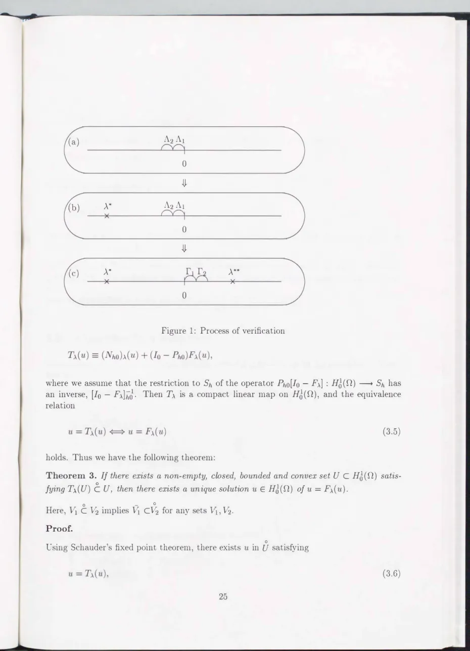
First, we assume that the ESAV is negative and we begin a procedure to determine a bound of ESAV moving from zero in the negative direction.

We consider a sufficiently narrow interval A

i

⁼⁼

( ai, ai-d,

^where

ai ( i � 1)

are negative real numbers and

a0 ==

⁰ (see Figure

1

(a)). For a fixed

i

and ).. E Ai, we consider

(3.3)

as the second-order elliptic boundary value problem. Then

(3.3)

has a trivial solution

u ==

^0.

Therefore, for any ).. E Ai, if we validate the uniqueness of the solution in

(3.3)

by the method described below, it implies that ).. is not an eigenvalue of

(3.3);

that is, there is no eigenvalue of

(3.3)

in Ai. If we fail to validate the uniqueness in an interval Aj , then we set).* ^_ infAj_1 (see Figure

1

(b)). Next, we start this procedure from zero and move the positive direction. In this case, if we fail to validate the uniqueness in an interval rk, _{then we} set ).. ** su pr k-1 (see Figure 1 (c)). Note that we can terminate this process when moving in the positive direction after infr1 > l-\*1 for some interval r1. By comparing the absolute value of ).. *and ). **, we can determine a lower bound for the ESAV.

If we fail to validate the uniqueness of the solution

u ==

⁰ in interval A1 or interval r _{1, this} implies that we could not get a bound of the ESAV as positive values. In this case, we must refine our method, for example, using a smaller mesh size or higher order base functions in Sh, etc. However, there is the possibility that

(3.3)

really has 0 as an eigenvalue in such a case.

Now, we describe a method to validate the uniqueness of solutions to

(3.3)

for a fixed ).. E _A

i

. Using the compact map on

HJ(D.)

we can rewrite

(3.3)

as

(3.4)

Then we set

0

JJ-

(b)

^{_\* A2 A1}

0

JJ-

(

c) ^_\*

�

^_\**

)( X

0

Figure ^1: Process of verification

where we assume that the restriction to

Sh

of the operator

Pho[Io- F"-] : HJ(D)

^----+

Sh

has an inverse,

[!0

^-

F"-]h"J.

Then T"- is a compact linear map on

HJ(D),

and the equivalence relation

(3.5)

holds. Thus we have the following theorem:

Theorem 3.

If there exists a non-empty) closed) bounded and convex set

U ^C

HJ(D) satis­

fying

^T;..(U)

C

U7

then there exists a unique solution u

^E

HJ(D) of u

⁼

F"-(u).

0 - 0

Here, V1 c V2 implies V1 cV2 for any sets Vi, V2.

Proof.

Using Schauder's fixed point theorem, there exists

u

in U satisfying 0

(3.6)

and by

(3.5)

it is equivalent to

u

⁼

F>. ( u).

Since

T>.

is a linear operator and T>-.

( u)

^{= u} holds, for any

c E

^{R we have}

cu. (3.7)

If

u

# 0, we can choose

c E

^R satisfying

cuE au.

But this contradicts with

T>.(U)

^C 0

U

and

(3.7).

Therefore

u

⁼ 0. That is,

u

⁼ 0 is a unique solution of

u

⁼

F>.(u). I

By Theorem

3,

if there exists a closed, bounded and convex set

U

^C

HJ(D.)

satisfying

U T>-.U C U

then it follows that the interval Ai contains no eigenvalues of

(3.3).

We use

>-.EAi

interval approaches to verify the condition

U T>-.U C U (cf.[14]).

>-EAi

3.3 Algorithm in

^a

computer

We now describe the actual computational procedures used to verify the condition in Theo­

rem

3.

For an interval vector

Bo

⁼

(BJ0))'f=1

and a strictly positive real number

a0,

^{we write}

where M = dim

Sh , ^{{ ¢j} }'f=1

is a basis of

Sh.

And we define

U

as

Then the verification conditions are written ^as follows:

{ (Nho)>-.(U) c uh

(Io- Pho)F>.(U) c U1_. (3.8)

M

L B1¢1

^:J

(Nho)>.U

j=l

and a real number ^a defined by

a=

Coh

sup

II(..\- q)viiL2

vEU satisfy the conditions

(3.9)

(3.10)

then the verification conditions

(3.8)

are satisfied, and there exists a unique solution of

(3.3)

in

U

for a fixed ,.\ E

Ai.

Note that the inclusion in the former part of

(3.10)

is meant componentwise.

Next we derive a necessary and sufficient condition for

(3.10)

which is simpler than

(3.10).

If

q

^{= ..\,}

(3.3)

has the only solution ^{u ==}

0.

Therefore we assume that

q t

^..\.

If we represent ^an element

v

in

U

as

V

⁼⁼

Vh

⁺

v 1_

for

Vh

^E

Uh

and

V

^{1_ E}

U 1_,

we have

That is,

( N hO) >. ( v h

⁺

v j_)

Pho(vh

⁺

v1_)- [Io- F>.]h5(Pho(vh

⁺

v1_)- PhoF>.(vh

⁺

v1_)) vh- [Io- F>.]h5(vh- PhoF>.(vh

⁺

v1_)).

[Io- F>.]hovh- (vh- PhoF>.(vh

⁺

v1_) ) PhoF>. ( vh

⁺

v 1_ ) - PhoF>. ( vh)

PhoF>.( v1_). ^(3.11)

To calculate the interval vector

(B1 )�1

satis

fy

^ing

(3.9),

we consider a set X such that

X =

{X

^E

^{sh I}

there exist ^{Vj_ E} uj_ such that, for all i =

1,

^{... , M,}

<

[Io- F>.]hox,q)i

>H1==< ⁰

PhoF>.(vl_),¢i

^>H10

}

^.

^(3.12)

In an actual computation, as shown below, we can obtain the interval hull of X

(

denoted by

I

^X

I )

by solving the linear system of equations in

(3.12)

using the interval right-hand side.

Therefore we can set

M

L:Bj¢j

⁼

W

^.

^(3.13)

j=l

Observe that for

¢i (1 :::;

ⁱ

:::; Jvf)

and

x

⁼

L:f=1 xi¢],

we have

(3.14)

and for all ^V1_ E U1_,

(3.15)

Therefore, in order to obtain the set

I

^X

I,

we define the

M

^x

M

matrix QC>..)

(g � ))1::;i,j::;M,

which is dependent on

A,

^by

g s ^A)

⁼

(\l¢i , \l¢j)£2 + (¢i , q¢j)£2-,\(¢i , ¢j)£2 (1::;

ⁱ ,

j:::; M)

and the interval vector

r

by

Since we supposed that

[Io -FJ\]hl

exists,

G(J\)

is invertible. Then, the interval coefficients

B1

in

(3.9)

are determined by

(3.16)

Note that B is obtained as the interval hull of the set

{ x

^E

RM I G(J\)x

⁼

a0r,

for all

r

^E

r}

by the usual interval arithmetic. We can estirnate

a

by using, for example, the triangle inequality

a C0h

sup

11(,\- q)vii£2

vEU

<

Coh {

^{VhEUh up}

11(,\-q)vhil£2+

^{V_LEU..L sup}

li(A-q)vl_ll£2 }

<

Coh

^sup

11(,\-q)vhll£2 + C6h2aoliA-qlloo,

VhEUh

where

II

^·

lloo

represents the L00-norm on .0. Then the following theorem holds.

Theorem

^4.

The conditions (3.1 0) are equivalent to the following inequality:

zE( G(.X) )-1 r

Proof.

First, we suppose that

(3.10)

hold. Then, the verification conditions

(3.10)

are written as

Thus we have

ao

>

Coh

_sup

11(-X- q)�t

^·

Boll£2

₊

C6h2aoii-X- qlloo

BoEBo

>

Coh

_sup

11(-X- q)if!t

^·

aozll£2

₊

C6h2aoii-X- qlloo

zE(G(.X))-1r

- no ( ^coh

zE(G(-A))-1r ^sup

11(-X- q)if!t

·

ziiL2

₊

C6h2II-X- qlloo ) ^,

and hence,

(3.17)

_holds.

On the other hand, suppose that

(3.17)

holds. Then defining

E-

1- Coh

_sup

11(-X- q)if!t

^·

zll£2- C6h2II-X- qlloo,

zE(G(-A))-1r

(3.18)

E >

0

_{holds by}

(3.17).

Since we assumed that

q

t A, we define the interval vector b0 as

bo

₌

T(M

₊

1)Cohii-X-

E

qlloo [1],

where

[1]

₌

([-1, 1], ... , [-1, 1])t, T

₌

l�i�M

_max

ll¢illu

and write

Then we have

(3.19)

and by straightforward calculation, we find that the following inequality holds:

Coh

sup

II(A- q)�t

^·

Boll£2

⁺

C6h2aoiiA- qlloo

<

ao.

BoEBo

This proves the theorem.

I

Remark 3.1

We can choose

ao

and Bo arbitrarily if they satisfy the relation

(3.19).

This arbitrarity comes from the linearity ofF>.., which enables us to calculate B independently of B0

(

See

(3.11)).

By Theorem

4,

if each

A

^E Ai satisfies

(3.17),

it follows that there is no eigenvalue of

(3.3)

in Ai. In our previous method

[14),

it is necessary to check the condition

(3.10)

in the sense of intervals. Actually, in that case we often failed to verify the uniqueness of the trivial solution on an interval in which no eigenvalues were contained. In the case of present method, the condition

(3.17)

can be easily checked for all

A

^E Ai. Thus, computational efficiency is greatly increased in our new method. This has been confirmed by actual computations.

There are two known methods to verify the existence of solutions of nonlinear elliptic equa­

tions, Nakao's method

[9-14)

and Plum's method

[17, 18).

In Nakao's method, one decom­

poses the equation into finite and infinite dimensional parts, and the former is processed by finite element approximations, while the latter is treated using constructive error estimates.

Then, Newton-like iterations for some function sets are executed to find a solution.

In Plum's method, the norm of the inverse of the linearized operator of the original differ­

ential equation is evaluated by rigorously estimating the Eigenvalue with Smallest Absolute Value (ESAV) of this linearized operator, and the solution in question is enclosed near an approximate solution by checking a condition of the Newton-Kantorovich type in an infi­

nite dimensional space. Therefore, in Plum's method the estimation of the ESAV plays an essentially important role.

In this section, we propose an alternative approach to this problem consisting of a mixture of Nakao's and Plum's verification 1nethods. More precisely, we use a form of Plum's method with local uniqueness for the basic formulation ( c

f. [25)),

and for the estimation of the ESAV of the linearized operator, we use Nakao's method described in Section 3. By applying such a mixed approach, we can obtain a new verification method which includes all the advantages of the two previous methods and none of their disadvantages.

4.1 Statement of the problem and the fixed point formulation

We consider the nonlinear elliptic boundary value problems of the form

{

^-6.

^u _u

^{= f (}

^u)

ⁱⁿ

^n'

= 0 on

an,

where we suppose that f satisfies the following assumptions:

Al. f :

HJ(D)

^---+

L2(D.)

is continuous and maps bounded sets into bounded sets.

A2. f is Fn§chet differentiable on

HJ(D).

Let

Uh

^E

sh

be a finite element approximate solution of

( 4.1)

satisfying

(

4.1)

We used the library PROFIL

(

^c

f. [4]),

which enables us to enclose the above

uh

in very small intervals. We attempt to find the solution of

(4.1)

near u satisfying

{ ^-

^!:::..

_u ^U

⁼

^{j (}

^{Uh) in}

^n,

= 0 on an.

( 4.2)

For this

u

E

H2(n) n HJ(n),

the relation

uh

⁼

Phou

holds, as can be confirmed by a simple calculation. From

( 4.1)

and

( 4.2),

we have

{

^-!:::..

⁽

^U

^{- U)}

⁼

^{j (}

^U

^{) - j (}

^{Uh) in}

^n,

u -

iL = 0 on an.

Defining

Vo

=

u-

uh, we then have v0 E

Sf:,

and we can write

Similar to the discussion in Section

2,

we obtain the following estimation:

Note also that in this estimation we used the L2-estimate of v0:

( 4.3)

Now, in order to verify solutions

u

of

( 4.1)

near

u,

writing w = u-

u,

we can rewrite

( 4.3)

as follows:

f(uh

⁺

Vo

^{+ w}

)

^-

f(uh)

0

inn, on an.

Let

(

-t:::..)-11/J be the solution of

(2.2)

for

1/J

E L

2(n) .

Then

is a bounded operator, and since the imbedding

H2(n)

^'---t

HJ(D)

is compact,

is a compact operator. Thu u ing the compact map F0

: HJ(D)

^---t

HJ(D)

defined by

( 4.4)

we have the fixed point equation for w on

HJ(n),

w

⁼⁼

Fo(w). ( 4.6)

Next, let

F6( -v0)

be the Frechet derivative of

F0

at

-v0,

and define

L

=

10 - F6( -v0).

Moreover, with

L

⁼

( -l:l)L: HJ(n)

^�

H-1(0.),

^by

F�( -v0)u

⁼⁼

( -l:l)-1 f'(uh)u,

^{we have}

which is a strongly elliptic operator. Here -� is interpreted in a distributional sense. Note that, by restricting the domain of definition of

L

^to

H2(n)

ⁿ

HJ(n),

we can regard the operator

L: HJ(n)

^�

H-1(0.)

^as

L: H2(n)

ⁿ

HJ(n)

^�

L2(n).

Now we discuss the existence of

L-1.

Since

L

₌₌

( -ll) (I o - F� (-vo))

holds,

( -�)-1 L

is a Fredholm operator of index 0. If the ESAV ).* of

L

is known to be nonzero, then we have the estimate

and therefore,

Lu

⁼⁼ 0 ¢::=::>

u

⁼⁼ 0,

which implies that

( -l:l)-1 L

is an injection. Thus by the Fredholm alternative theorem,

( -l:l)-1 L

has an inverse. Hence the existence of the continuous operator

L -1 : L2(0.)

^�

H2(D.)

ⁿ

HJ(D.)

is confirmed.

Now, define the operator

T0 : HJ(n)

^�

HJ(n)

as follows:

( 4.7)

This operator is derived by a Newton-like method for the equation

(10 - F0)w

⁼

0.

Then, since the imbedding

H2(f2)

^Co.-...t

HJ(D)

is compact, using assumptions Aland A2,

To

becomes a compact operator on

HJ ( n),

and we have

w

⁼

To(w)

<===>

w

⁼

Fo(w).

4.2 Verification conditions

In this subsection we present a verification condition with uniqueness based upon

[25).

Now, we intend to find a solution to

(4.1)

in a set

W0.

Taking a strictly positive real number

a,

a candidate set

W0

is defined by

( 4.8)

By the method described below we choose strictly positive constants f3 and 1 such that

II To ( 0) II H 6 :::; f3 , ( 4.9)

for all

w1, w2 E Wo. (4.10)

We then define the set

K0

c

HJ(n)

by

Ko={vEHJ(n) lllviiHJ :::;{3+!}, ( 4.11)

which includes the image of

W0

transformed by the linearized operator of

T0.

The verification condition is described in the following theorem.

Theorem 5.

If Ko

C

Wo holds for a candidate set W0 defined by (4.8), namely,

f3 +!:::;a, (4.12)

then there exists a solution to { 4.1) in u + K0. Moreover, this solution is unique within the set u+

Wo.

Since the proof of this theorern is similar to that of Theorem

1,

we describe the outline of it.

Outline of proof.

We define a caling norm

II

^·

II

w0 by

where ^a is the same one in

( 4.8).

Using this norm we can prove that

To(Wo)

C

Wo

and

for some k s.t.

0

^< k ^<

1

and for all w1, w2 E

W 0

. Then we can apply Banach's fixed point theorem to obtain the desired conclusion.

1

4.3 Estimation of constants and algorithm

In this subsection we describe the n1anner in which the constants in

( 4.9)

and

( 4.10)

are obtained.

Constant {3

Since

holds, we consider constants (1 and 17 satisfying

IITo(O)IIHJ � (111f(uh

+

vo)- f(uh)il£2, llf(uh

+

vo)- f(uh)li£2 _�

17·

We then can choose {3 to be

(177.

As for (1 we first calculate the constant

(o

such that

This constant

(0

is obtained ^as the inverse of the ESAV of

(4.13) ( 4.14)

(4.15)

( -6.)Lu

⁼

>..u.

(4.16)

Then we can calculate

(1

from

(o

as follows ( cf.[17]). Assume that

L00(D)

3

q

⁼

_- f'(

^uh

)

and that there exist constants

g_, ^q

such that

9_ � q( X) � q (X

E

f2).

Then the constant

(1

is derived as follows:

(1

⁼

1 V(o(1- g_(o) ₁

^if

g_(o ^� �'

-- otherwise.

2�

( 4.17)

(4.18)

Since

f(·)

E

L2(D)

is assumed to be bounded, TJ can be calculated using a simple estimation.

Constant 1

We consider a constant

(2

and a monotonically increasing function

Q

:

[0,

oo

)

---+

[0,

oo

)

such that for all

w1, w2

E

Wo,

( 4.19) ( 4.20) Then since we have

we can choose 1 as

(2Q(cx).

As for

(2,

since

holds for all

w1 w2

E

W0,

we can choose

(2

⁼

(1.

vVith regard to the monotonically increasing function

Q

since

f'

:

HJ(D)

^�

.C(HJ(D), L2(D))

(the space of bounded and linear operators

HJ(D)

^�

L2(D))

is a bounded and linear operator, we can construct

Q

as

Now, we describe an algorithm for finding a real number

a

which satisfies the verification condition

( 4.12),

Since 1 depends on

a,

we write 1 as

I=

!(a).

If f

(

u

)

in

( 4.1)

is a polynomial in u,

!(a)

is a polynomial in

a.

Therefore, in order to find

a

satisfying

( 4.12),

we may solve the inequality for

a.

Here we present the following iteration method.

Algorithm

1.

Fix a maximum iteration number.

2.

Find a constant {3 satisfying

( 4.9).

3.

Set

a� _{3.

4.

Find a constant

!(a)

satisfying

(4.10).

5. Check the verification condition

(4.12); _{3 +!(a)::; a.

If the condition is satisfied, the verification has succeeded. If not,

Set

a� (1 +8)a (0

<

8

<<

1), (4.21)

where

8 (0

^<

8

<<

1)

represents an inflation parameter

(cf.[19],[23]

etc.). Then increase the iteration number by

1

and return to step

4.

6. If the maximum iteration number is exceeded, without

( 4.12)

being satisfied, the verification has failed.

5 Numerical examples

First, we give two examples whose eigenvalues were enclosed using the method in Section

2.

Specifically, we have verified the eigenvalues with the smallest absolute values

(

ESAV) with the technique described in Section 3. We set the following conditions:

n is the rectangular domain

(0, 1)

^X

(0, 1)

^c

R2'

and the interval

(0,1)

was partitioned into

20

pieces

(

^{h =} 210

)

^. The basis in S

h

consists of continuous, piecewise biquadratic polynomials on n.

(M

⁼ dimSh ⁼

1521)

The inflation parameter 8 in

(2.40)

is set to

0.0001.

Then the constants appearing previously can be taken as

cl

^{= 2}

�

^and

^c2

⁼

1 ( cf.[14]).

In the calculations, interval arithmetic is used to avoid the effects of rounding errors in the floating-point computations. The computations were carried out on a Sun Enterprise

450

using the interval library PROFIL coded by Kniippel of the Technical University of Hamburg-Harburg

([4]).

PROFIL is implemented as a portable C++ class fast interval library and supports two interval solvers proposed by Rump

([19]).

Example 1:

We consider the following self-adjoint eigenvalue problem:

{ -flu- 2uhlu

^{= AU inn,}

u

⁼

0

on an,

(5.1)

where

uh1

is a finite element solution of the following so-called Emden equation:

{ ^-flu _u

⁼

^u2

^{in n,}

=

0

on an.

(5

^.

2)

We calculated a finite element approximate solution

(uh, ):h)

satisfying

(2.6)

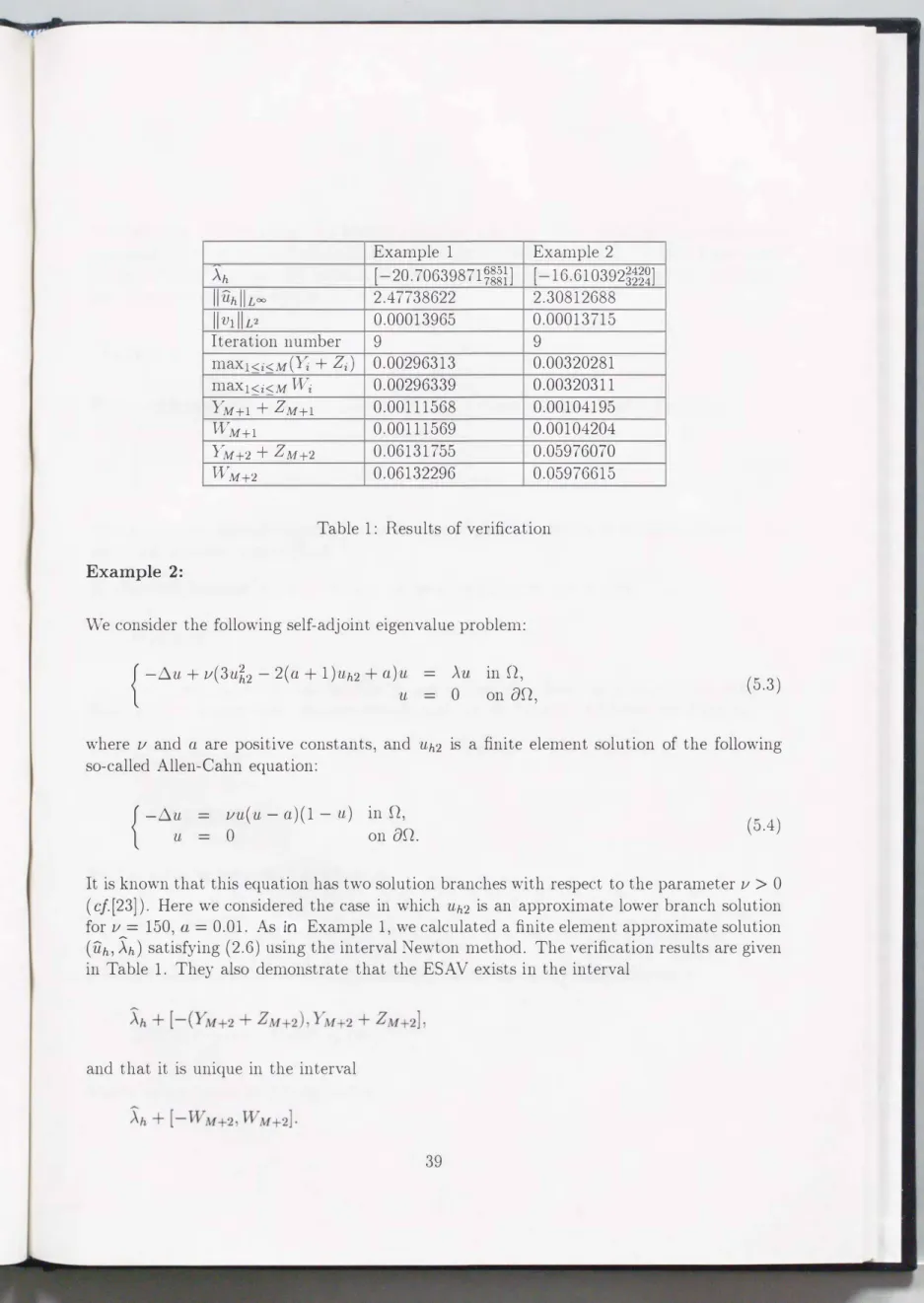
using the interval Newton method. The verified results for the ESAV are given in Table

1.

These demonstrate that the ESAV exists in the interval

and that it is unique in the interval