Finite Element
Approximations of
Conformal Mappings
Takaya
TSUCHIYA
(
土屋卓也
)
Department of Mathematical Sciences
Faculty ofScience
Ellinle University
Matsuyama 79ti-8577, JAPAN
[email protected]. ehime-u.$\mathrm{a}\mathrm{c}\cdot.\mathrm{j}\mathrm{p}$
Abstract. In this paper, finite element approximations of $\mathrm{c}.\mathrm{o}\mathrm{n}\mathrm{f}\mathrm{o}\mathrm{r}\mathrm{n}\mathrm{l}\mathrm{a}^{]}\sim \mathrm{I}\mathrm{n}\mathrm{a}_{1^{)}}\mathrm{I}^{)}\mathrm{i}\mathrm{n}\mathrm{g}\mathrm{s}$
defined on the unit disk to Jordan regions are $\mathrm{c}\mathrm{o}\mathrm{n}\mathrm{s}\mathrm{i}\mathrm{d}\rho \mathrm{r}\mathrm{e}\mathrm{d}$. Three types of$\mathrm{t}1\mathrm{l}\mathrm{e}\mathrm{n}\mathrm{o}1’ \mathrm{I}\iota 1\dot{\mathrm{c}}\mathrm{i}\neg..1\mathrm{i}’/_{\lrcorner}\mathrm{a}-$
tion conditions are dealt with. In each case, convergence of the fillite $\mathrm{e}\mathrm{l}\mathrm{e}\mathrm{I}\mathrm{n}\mathrm{e}\mathrm{n}\mathrm{t}_{\mathrm{C}\mathrm{o}\mathrm{r}}1\mathrm{f}\mathrm{o}\mathrm{J}Y\mathrm{m}\mathrm{a}^{1}1$
mappings to the exact solution isproved.
1.
Introduction.
Let $D\subset \mathbb{R}^{2}$ be the unit disk, $\mathrm{a}\ovalbox{\tt\small REJECT}\Omega\subset \mathbb{R}^{2}\mathrm{a}_{}$ bounded
$(1\mathrm{o}\mathrm{m}_{\zeta}\eta\dot{\mathrm{n}}\mathrm{i}\mathrm{m}\backslash \mathrm{v}\mathrm{h}‘)\mathrm{l}\Re \mathrm{t}_{)\mathrm{O}}\mathrm{u}\mathrm{n}\mathrm{d}_{\nu}^{\}}\mathrm{a}\mathrm{W}^{\partial.?}\langle^{-}$ is a closed JorelaIl
curve
$\wedge/\subset \mathbb{R}^{2i}${slkM
$\mathrm{I}\mathrm{b}\#$)$\Psi^{(\mathrm{m}}\oplus$($*_{\backslash }$ regiums
$\mathrm{a}\mathfrak{B}ffl^{\}}\mathrm{c}\mathrm{a}]\#\mathrm{b}_{\mathrm{C}d}\downarrow.J\acute{O}\mathit{1}\iota’ d\mathrm{a}\mathrm{m}\Gamma \mathrm{A}\tau gi\langle$)
$R4’)\neg$. Let
$\varphi$ :
$\overline{D}arrow\overline{\Omega},$ $\varphi\in c(\overline{D}:\mathbb{R}\underline{9})|\cap c^{3}\mathrm{p}D;\mathbb{R}‘\eta_{\mathfrak{b}_{\Psi}}c^{1}\triangleleft 1\dot{\mathrm{u}}\mathrm{f}\mathrm{f}\mathrm{l}oe(\zeta)\mathrm{i}\mathrm{m}\varpi \mathrm{n}1i)\mathrm{A}\dot{\mathbb{I}}\mathrm{R}$ alud$! $\mathrm{i}_{\mathfrak{B}}$
$\mathrm{o}\mathrm{n}1\mathrm{u}\mathrm{t},\ovalbox{\tt\small REJECT}\dot{\mathrm{O}}\mathrm{n}_{\mathrm{P}^{\mathrm{r}\mathrm{e}}\mathrm{g}}\succ \mathrm{s}\mathrm{e}\mathrm{r}\mathrm{V}\mathrm{i}\mathrm{n}$ .
If $\varphi$ also preserves any angks of two
curves
crossing $\mathrm{a}f$ a point in $D,$$\varphi$ is
$\mathrm{c}\mathrm{a}^{1}|\wedge]_{\mathrm{G}(\rfloor}$ a
conform$\mathrm{a}l$ mappin
$g$. $\mathrm{F}\mathrm{r}\mathrm{o}111$
the theory of complex $\mathrm{f}\mathrm{u}\mathrm{n}\mathrm{c}\cdot \mathrm{t}\mathrm{i}_{0}11\mathrm{s}$, we know $\mathrm{t}\mathrm{h}_{\dot{\epsilon}}\iota \mathrm{t},\dot{\mathrm{J}}\mathrm{f}c\mathrm{J}\zeta^{\gamma\rceil},.$.
diffeomorphism $\varphi=(\varphi_{1}, \varphi_{2})$ : $Darrow\Omega$ is conformal, $\mathrm{t}\mathrm{I}_{\mathrm{l}\mathrm{e}}11\mathrm{t},1_{1\mathrm{C}}\mathrm{C}\mathrm{o}\mathrm{m}_{\mathrm{I})_{\mathrm{A}}\mathrm{e}}1\mathrm{X}^{- \mathrm{v}_{C})}‘ 1\mathrm{u}\mathrm{e}\mathrm{d}\mathrm{f}\mathrm{u}\mathrm{n}\mathrm{c}\mathrm{t}\mathrm{i}\mathrm{I}^{-}$ ) $\iota 1$
$f(z):=\varphi_{1}(x_{1\mathrm{t}}X_{2})+\sqrt{-1}\varphi_{2}(:r1, X2)$ is differentiable with
$1^{\cdot}\mathrm{e}\mathrm{s}_{1}$) $\mathrm{f}^{1}(\urcorner \mathrm{t}.$
. to the $(^{\tau}\mathrm{o}\mathrm{n}1\}^{)}1\mathrm{C}\mathrm{X}$ value
$z:=.x_{1}+\sqrt{-1}x_{-}‘)$, and vice versa. Ill $\mathrm{t}1_{1}\mathrm{i}\mathrm{s}$ paper, we study fillitC
$\mathrm{e}\mathrm{l}\mathrm{e}\mathrm{l}\mathrm{l}\mathrm{l}\mathrm{e}\mathrm{l}\mathrm{l}\dagger \mathrm{a}_{1^{)}1^{)\mathrm{r}\mathrm{t}_{\grave{\text{ノ}}}}}\mathrm{X}\mathrm{i}_{1I}1\mathrm{a}\uparrow \mathrm{i}_{01}1$
ofconformal $\mathrm{n}\mathrm{u}\mathrm{a}_{\mathrm{P}\mathrm{P}^{\mathrm{i}_{1}i\supset}}\mathrm{l}\mathrm{g}$’ on th$t^{1}$ ullit disk.
For$\mathrm{c}\mathrm{o}\mathrm{I}\mathrm{l}\mathrm{f}_{0}\mathrm{r}\mathrm{l}\mathrm{n}\mathrm{a}\mathrm{l}\mathrm{n}\mathrm{l}\mathrm{a}\mathrm{I}^{)}1$)$\mathrm{i}_{\mathrm{I}}1\mathrm{g}\mathrm{s}\mathrm{f}_{\mathrm{f}\mathrm{O}\mathrm{I}}\mathrm{n}$the unit disk to Jordan
$\mathrm{r}\mathrm{e}^{1}\mathrm{g}\mathrm{i}\mathrm{o}\mathrm{n}\mathrm{k}\backslash$” the
$\mathrm{f}\mathrm{o}11\mathrm{o}\mathrm{w}\mathrm{i}_{\mathrm{I}}\iota_{\mathrm{o}}\sigma_{\mathrm{V}}\mathrm{a}\mathrm{r}\mathrm{i}\mathrm{a}\mathrm{t}\mathrm{i}_{01}1‘ \mathrm{a}$\‘i $\mathrm{I})\mathrm{r}\mathrm{i}\mathrm{n}\mathrm{c}\mathrm{i}\mathrm{p}\mathrm{l}\mathrm{e}$ has been known (for example,
see [3, pp. 107-115], [4, Section 4.5]): $\mathrm{I}$)$\mathrm{e}\mathrm{f}\mathrm{i}\mathrm{l}\mathrm{l}\mathrm{G}$ the
subset $X_{\gamma}$ of$C(\overline{D};\mathbb{R}2)\cap H^{1}(D;\mathbb{R}^{2})$ by
(1.1) $X_{\gamma}:=\{\psi\in C(\overline{D};\mathbb{R}^{\angle})’\cap H^{1/}(D;\mathbb{R}2)|\eta’’(_{\backslash }\partial D)=\wedge/‘ \mathrm{a}\mathrm{n}\mathrm{d}\psi|_{)D}$
where $\psi|_{\partial D}$ being monotone $\mathrm{m}\mathrm{e}‘ \mathrm{a}11\mathrm{S}$ that
$\eta$)$|_{\partial D}$ preserves
$\mathrm{t}fi\mathrm{e}\mathrm{o}\mathrm{r}\mathrm{i}_{\mathrm{C}\mathrm{I}}1\mathrm{t}\mathrm{a}\mathrm{t}\mathrm{i}(11$ of $\partial D$, and $(\psi|_{\partial D})^{-}1(p)$ is connected for any $p\in \mathrm{A}(\cdot$ We denote the Dirichlet integral (or
$\iota 1\mathrm{j}\mathrm{C}^{\backslash }(^{\mathrm{Y}}11-$ ergy functional) on $D$ for $\varphi=(\varphi_{1}, \varphi_{2})\in H^{1}(D;\mathbb{R}^{2})$ by
(1.2) $D( \varphi):=/D|\nabla\varphi|^{2}dx=\int_{D}(|\nabla\varphi_{1}|^{2}+|\nabla\varphi_{2}|^{2})d.\iota:$.
Then, we have that $\varphi\in X_{\gamma}$ is $con\mathrm{f}_{oTl}\mathit{1}1al$ if and $onl_{V}$
. if$\varphi\in X_{\gamma}$ is a $\mathrm{s}\mathrm{t}\partial$tion
$\dot{‘}u\cdot.$)’ poin
$\mathrm{f}$ of$\mathrm{t}b\mathrm{c}^{1}$
functional $D(\varphi)$ in $X_{\gamma}$. The problen] of finding stationary points oftlle
$\mathrm{I}$)$\mathrm{i}\mathrm{r}\mathrm{i}\mathrm{C}\mathrm{h}$]
$\mathrm{e}\{\mathrm{i}_{1\perp \mathrm{t}\mathrm{g}}(^{}\underline{1}^{-}\mathrm{a}1$
in $X_{\gamma}$ is called the Plateau problem [3], [4]. Therefore, in this sense, the corlforlnal
mappings are minimal surfaces in $\mathbb{R}^{2}$
.
By the Riemann mapping theorelll, or the existence proof of solutions of the $\mathrm{P}1_{\mathrm{d}}\mathrm{t}\mathrm{e}‘ \mathrm{C}m$
problem, there exist $\mathrm{C}\mathrm{o}\mathrm{n}\mathrm{f}\mathrm{o}\mathrm{r}\mathrm{m}\mathrm{a}\mathrm{l}_{\mathrm{l}\mathrm{n}\mathrm{a}\mathrm{p}\mathrm{P}}\mathrm{i}\mathrm{n}\mathrm{g}\mathrm{L}\mathrm{s}’\varphi\in X_{\gamma}$, and we have
$D(\varphi)=,\mathrm{i}_{1}\mathrm{v}_{\sim}^{\epsilon^{1}}X\mathrm{f}\gamma D(\psi)=|\Omega|$,
where $|\Omega|$ is the area of$\Omega$. It is also well-known that in our casethe $(^{\backslash }(\mathrm{n}\mathrm{f}_{0}\mathrm{r}1\iota 1_{C}‘:\iota 1_{11}1‘ \mathrm{d}\mathrm{I})1^{\mathrm{i}\mathrm{n}\mathrm{g}_{\mathrm{b}}})\mathrm{f}\mathrm{i}$
are homeomorphisms between $\overline{D}$
and $\overline{\Omega}$
.
To specify a conformal mapping, we need a normalization condition. Several
normal-ization conditions are known for conformal $\mathrm{m}\mathrm{a}\mathrm{p}\mathrm{I}^{)}\mathrm{i}_{1}_{\mathrm{S}}$on the unit disk. Ill this papei. $\mathrm{W}^{(^{1}}$
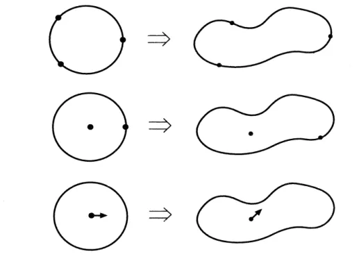
deal with the following conditions (see Figure 1):
$\supset$
$\Rightarrow$
$\Rightarrow$
Figure 1: The three normalization conditions.
(a) Specify the image of three points $011\partial D$.
(c) Specify the image of a point in $D$ and the direction of derivative at the point.
In the following sections we discuss finite element approxinlations of$\mathrm{c}\mathrm{o}\mathrm{n}\mathrm{f}_{0}\mathrm{r}\mathrm{l}\mathrm{n}\mathrm{a}1$
map-pings with the above normalization conditions. Since the number of pages is linlited. we
cannot give any numerical examples in this article. They and a detailed $\mathrm{d}\mathrm{i}\mathrm{S}\langle \mathfrak{U}_{\backslash }\mathrm{q}\mathrm{s}\mathrm{i}\mathrm{o}\mathrm{n}$ on
implementation of finite element conformal mappings will be given in the finalversion of
this paper.
2.
Finite
element
approximation of conformal
map-pings
In this section, weconsider afinite element approximation ofconformal mappings. First,
we suppose that we have a family of regular triangulation $\{\triangle_{h}\}$ of’ the unit disk with
triangles (for the definition of regular tnangula,tion see Ciarlet [1, p124]). wllere $h\mathrm{S}\mathrm{t}\mathrm{a}11\mathrm{d}_{\mathrm{S}}$
for the maximum size of triangles in the triangulation $\triangle_{h}$, and $harrow \mathrm{O}$. Set $D_{l\iota}$ $:=$
$\bigcup_{K\in\triangle_{h}}K$. Note that $D_{h}\subset D$ for any $h$. Let $S_{h}\subset c^{0}(D_{\iota},)$ be the set of piecewise linear
functions on each triangle. We extend the functions of $S_{h}$ in the following mallller. On
a point $x\in\partial D_{h}$, which is not a nodal point, there exists an outer $\mathrm{n}\mathrm{o}\mathrm{l}\cdot \mathrm{m}\mathrm{a}\mathrm{l}$ half line $f$. On
$y\in l\cap(D-D_{h})$, the value of $f_{h}\in S_{\iota}$
,
is defined by $f_{h}(y):=f_{h}(x)$. A straightforwardcomputation yields
$\int_{D_{h}}|\nabla v_{h}|^{2}dX\leq\int_{D}|\nabla v_{j\iota}|^{2}dX\leq(1+Ch)[\mathrm{t}D_{h}|\nabla v_{h}|^{2}dX$
for any $v_{h}\in S_{h}$, where $C$ is a positive constant independent of$h$.
We discretize $X_{\gamma}$ as
$\mathrm{S}_{\gamma,h}:=\{\psi_{h}\in(S_{h})^{2}|\tau f_{J}h(\partial D\cap N_{h})\subset\gamma$ and $\psi_{h}|_{\partial D}$ is $d- \mathrm{m}\mathrm{o}\mathrm{l}\mathrm{l}\mathrm{o}\mathrm{t}\mathrm{o}\mathrm{n}\mathrm{e}\}$,
where $N_{h}$ is the set of nodal points ill $D_{h}$, and $\psi_{h}|_{\partial D}$ being $d$-lnonotone means that the
order of nodes on $\partial D$ is preserved on
$\gamma$ by $\psi_{h}|_{\partial D}$.
The finite $\mathrm{e}l\mathrm{e}m\mathrm{e}nt$ (or $FE$) $Conf_{orl}\mathrm{n}al$ mappings $\varphi_{h}$ are defined as the Ininimizer of
the Dirichlet integral $D(v_{h})$ in $\mathrm{S}_{\gamma,h}$:
$D( \varphi_{/\iota})=\inf_{hv_{h}\in \mathrm{S}\gamma},D(\mathrm{C}\prime h)$.
Since$\mathrm{S}_{\gamma,h}$ isasubset offinite-dimensionalEuclidean space, it is obvious that FE conformal
mappings exist.
From the definition it is obvious $\mathrm{t}_{J}\mathrm{h}_{\partial}\mathrm{t}$ finite elelnent conformal mappings are ‘$(1\mathrm{i}_{\mathrm{S}\mathrm{c}}\mathrm{r}\mathrm{e}\{\mathrm{e}$
$\mathrm{h}\mathrm{a}\mathrm{r}\mathrm{n}\mathrm{u}\mathrm{o}\mathrm{n}\mathrm{i}_{\mathrm{C}}1\mathrm{n}\mathrm{a}\mathrm{p}\mathrm{P}^{\mathrm{i}\mathrm{g}}\mathrm{n}\mathrm{S}.$” That is, if$\varphi_{h}\in \mathrm{S}_{\gamma,h}$ is a FE conformal mapping. $\varphi_{h}$ isthe
$\mathrm{m}\mathrm{i}\mathrm{n}\mathrm{i}_{1}\mathrm{n}\mathrm{i}\mathrm{z}\mathrm{e}\mathrm{r}$
is the unique solution of the weak problem
(2.1) $\int_{D}(\nabla\varphi_{h}^{1}\cdot\nabla v_{h}^{1}+\nabla\varphi_{h}^{2}\cdot\nabla v_{h}^{2})dx=0$ , $\forall v_{h}\in \mathrm{S}_{h}^{0}$,
where $\mathrm{S}_{h}^{0}$ is defined by
$\mathrm{S}_{h}^{0}:=\{v_{h}\in(S_{h})^{2}|v_{h}=0\mathrm{o}\mathrm{n}\partialarrow D\}$.
It is well-known that the maximum principle does not hold for discrete harmonic
mappings in general. We however have the following weak $m$aximum $pri\mathrm{n}$ciple for thc
discrete harmonic mappings proved by Schatz [5]:
Lemma 2.1 Let the triangulation $\{\triangle/l\}$ be regular and quasi-uniform. Suppo.se that
$\varphi_{h}\in \mathrm{S}_{\gamma,h}$
satisfies
(2.1). Thenfor
sufficiently small $h$ there exists a $\mathit{1}’?osifi?$)$CC\geq 1$independent
of
$h$ and $\varphi_{h}$ such that(2.2) $||\varphi h||_{L}\infty(D)\leq C||\varphi_{h}||_{L^{\infty}(D)}\partial$. $\square$
3.
The Three Point Condition
In this section we consider the first normalization condition. Let $z_{1},$ $\approx_{2},$$\approx \mathrm{s}\in\partial D$ and
$\zeta_{1},$$\zeta_{2},$$\zeta_{3}\in\gamma$ be taken so that those points define the salne orientation on $\partial D$ and $\gamma$.
Define
$X_{\wedge}^{tp},:=\{\psi\in X_{n_{\mathcal{P}}}|\psi(z_{i})=\zeta_{i},$ $i=1,2,3\}$
.
where “
$tp$” stands for the three point condition. It is obvious that
$\inf_{\psi\in X_{\gamma}^{tp}}D(\psi)=\inf_{\psi\in \mathrm{x}_{\gamma}}D(\psi)$.
By the Riemann mapping theorem we have
Theorem 3.1 There exists a unique $\varphi\in X_{\gamma}^{tp}$ which is
conformal
and $bi_{J^{eC}}t^{J}\iota’\prime ebet_{I\ell)}ee\eta$$D$ and $\Omega$. Moreover, $\varphi$ :
$\overline{D}arrow\overline{\Omega}$
is a homeomorphism. $\square$
To prove Theorem 3.1 we use the following well-known lemlna [3, Lennna $.‘ \mathit{3}.\underline{9}_{\rfloor}^{\rceil},$ $[4$
.
Section 4.3]:
Lemma 3.2 Let $M$ be a positive constant such that the subset $A\subset X_{\gamma}^{tp}$
defined
by$A:=\{\psi\in X_{\gamma}^{tp}|D(\psi)\leq M\}$
Therefore, takingaminimizing sequence $\{\psi_{7l}^{l}\}n=1\infty$ suchthat $\lim_{narrow\infty}D(?f_{\eta}))=\inf_{\lambda_{\wedge}^{tp}}.D(\emptyset)$
.
it follows from Ascoli-Arzel\‘a’s theorem that there exists a subsequence $\{\psi_{n_{i}}\}$ such thatj
$\{\psi_{n_{i}}|_{\partial D}\}$ converges some $g\in C(\partial D;\mathbb{R}2)$ uniformly. Moreover, from the lower
semi-continuityofthe Dirichlet integral, we conclude that the solution $\varphi\in X_{\gamma}^{tp}$ ofthe Laplace
equation
$\triangle\varphi=0$ in $D$, $\Psi^{\prime\cap=g}$ on $\partial D$
is the desired conformal mapping.
We follow the above scenario to define the finite element conformal mappings. Let
$\{\triangle_{h}\}_{h>}0$ be a family ofregular triangulation of the unit disk such that $harrow \mathrm{O}$. In this
section we always suppose that the point $z_{1},$$z_{2},$$z_{\mathrm{s}}\in\partial D$ are nodal points of $\triangle_{h}$ for each
$h>0$. Define the subset $\mathrm{S}_{\gamma,h}^{tp}$ by
$\mathrm{S}_{\gamma,h}^{tp}:=\{\psi_{h}\in \mathrm{S}_{\gamma,h}|\psi h(Z_{i})=\mathrm{G},\dot{\}.=t,$ $2,3^{\cdot}\}$.
Definition 3.3 A map$\varphi_{h}\in \mathrm{S}_{\gamma,h}^{tp}$ is called the
ffnite
element $conf\sigma rmaP$mappingif
it is a minimizer
of
the Dirichlet integral in $\mathrm{S}_{\gamma_{\backslash }h}^{tp}$:$D( \varphi_{h})=\inf_{\mathrm{r}_{\gamma}^{tp}\iota\dot{J}\prime\iota\in h},D(\psi_{h}\cap)$. $\square$
We nowconsider the convergenceof the finite element conformal$\mathrm{n}\mathrm{l}\mathrm{a}\mathrm{p}1$)
$\mathrm{i}\mathrm{n}\mathrm{g}_{\mathrm{S}}$. For each
$h>0$ there exists a finite element conformal mapping $\varphi_{h}\in \mathbb{S}_{\gamma,h}^{tp}$. The following is $\mathrm{t}\}_{1\mathrm{e}}$
most crucial [8, Corollary 8]:
Lemma 3.4 Let $\{\Delta_{h}\}_{h>}\alpha k$, afamily
of
regular tnangnlationof
the unit disk such that$harrow \mathrm{O}$ and
$z_{\mathrm{I}},$ $z_{2,3}Z\in\partial D$ are nodafpoints$\mathfrak{M}l\triangle_{h},fo7^{\cdot}$ cach$h>()..s_{uppos}e\iota\downarrow hat$, the Jordan
curve $\gamma$ is
rectifiabte.
$Then_{7}$for
$t!htese_{\mathfrak{M}^{e\tau b}}$ceof
thefinite
$elem/ew(lwJn^{\backslash }f_{1}ormw\# m/\cdot appings$$\{\varphi_{h}\}_{h>\circ}$, the
function
$\{\varphi_{h}|_{\partial D}\}_{h>0}$ are $cq^{\prime ui,cnt}in^{J}\alpha ous$ on $\dot{c}$)$D$. $\coprod|$By the exactly same mallner as ill [7] we obtain
Theorem 3.5 Let $\{\triangle_{h}\}_{h>0}$ be a family
of
$regula\uparrow\cdot q\mathrm{t}\iota a\mathit{8}i$-uniform
tnangulationof
the unitdisk such that $harrow \mathrm{O}and\approx_{1},$$\approx_{\mathit{2}}‘,$$z_{3}\in\partial D$ are nodal $p_{oin}t_{/}\mathit{8}7n\triangle_{h}$
for
each $h>0$. Supposethat the Jordan curve $\wedge$
[ is
rectifiable.
$Then_{y}$ the sequenceof
thefinite
$eler\prime e\gamma tt$ (.onformalmappings $\{\varphi_{f_{l}}\}_{h>0}$ converges to the exact
conformal
$mapp\uparrow ng\hat{\Psi}’\in\lambda_{\gamma}^{\prime 1}p$ in thefolfo
$\tau\iota’ ing$$\backslash \mathrm{s}ense$:
$\lim_{\prime\iotaarrow 0}||\Psi^{\cap}-\varphi_{h}||H^{1}(D,\mathrm{P}\mathrm{L}\underline{)})=0$.
and
if
$\varphi\in \mathrm{M}^{1,p}’\gamma(D;\mathbb{R}^{2}),$ $p>2$, then$\lim_{harrow()}||\varphi-\varphi_{h}||(_{\text{ノ}^{}\gamma}(o,\mathbb{P}^{2})=0.$
Remark In [7], [8], the family $\{\triangle_{h}\}_{h>}0$ of triangulation was supposed to be of $l\mathit{1}$
on-negative type (see [2]) to ensure the maximum principle for the discrete harmonic $\mathrm{m}\mathrm{a}_{1^{)-}}$
pings. However, since the weak maximumprincipleprovedbySchatz (Lemma2.1) is good
enough for our proof, we only needto assume tllat $\{\triangle_{h}\}_{l_{l>}0}$ is quasi-uniform instead. $\square$
4. The
One
Point
Condition
In this sectionwe consider another normalization condition: the on$e$poillt $col1$dition. Let
$z_{0}\in D$ and $\zeta_{0}\in\Omega$. Define $X_{\gamma}^{op}$ by
$X_{\gamma}^{op}:=\{\psi_{\in x}\gamma|\psi(\sim 70)=(_{0\}}$.
We know that the degree of “freedom” of conformal mappings in $X_{\gamma}^{op}\mathrm{i}_{\backslash }\backslash ^{\backslash }$ just
$\mathrm{o}\mathrm{n}\mathrm{e}_{i}\mathrm{a}\mathrm{l}1(1$
if rotation around $z_{0}$ is specified, then the conformal $\mathrm{m}\mathrm{a}_{\mathrm{I}^{)}\mathrm{P}^{\mathrm{i}\mathrm{n}}\mathrm{g}}$ is determined uniquel.$\mathrm{v}$.
As is stated in Section 1 we specify either the correspondence ofboundary $\mathrm{p}\mathrm{o}\mathrm{i}_{1}1\mathrm{t}\mathrm{S}$ or the
direction of the derivative at $\sim’ 0$ to fix rotation.
To take the same strategy as in Section 3, we would have to $1$)$\mathrm{r}\mathrm{o}\mathrm{v}\mathrm{e}$ that, for a positive
constant $M>|\Omega|$ and the subset $A:=\{\psi\in X_{\gamma}^{op}|I\mathit{3}(\psi_{J})\leq M\}$, the functions $\{\nu^{\mathit{1}}|_{\mathrm{C}}‘)D\}\psi\in A$
are equicontinuous. It seems, however, that this lnay be a wrong $\mathrm{s}\mathrm{t}\mathrm{a}\mathrm{t}\mathrm{e}\mathrm{n}\mathrm{l}(\supset \mathrm{n}\mathrm{t}$ . Thus, wc
must impose an additional condition to make it valid.
A mapping $\psi\in X_{\gamma}$ is called $l\mathrm{n}$onotone if $\psi^{-1}(p)\subset D$ is connectecl for any $1$)
$\mathrm{o}\mathrm{i}\mathrm{n}\tau$
$p\in\psi(D)$. We redefine $X_{\gamma}^{op}$ by
$X_{\gamma}^{op}:=\{\psi\in X_{\gamma}|\psi(z\mathrm{o})=(0$ and $\psi$ is morl$o\mathrm{t}_{0}11\mathrm{e}\}$.
Then we have
Lemma 4.1 Let $M$ be a positive constant such that $M>|\Omega|$. $Let-4:=\{\psi’\in X_{\gamma}^{op}|$
$D(\psi)\leq\Lambda_{i}\mathrm{f}\}$. Then the
functions
{
$\psi|_{\partial D\}_{\psi\in A}}$ are equicontinuous.Proof.
First, we recall the famous Courant-Lebesgue lemma [3, pp.101-102], [4,Sec-tion4.4]. For any $z\in \mathbb{R}^{2}$ and any $r>0$ we define
$S_{r,z}:=D\mathrm{n}\{w\in \mathbb{R}^{2} : |w-z|<r\}$, $C_{r,z}:=\overline{D}\mathrm{n}\{w\in \mathbb{R}^{2} : |\mathrm{t}\mathrm{t}^{)}-Z|=\gamma\}$.
If $z\in\partial D$, then we can write
$C_{r,z}=\{z+re^{i\theta} : \theta_{1}(r)\leq\theta\leq\theta_{2}(r)\}$ with $0<\theta_{1}(r)-\theta_{\wedge}‘)(7^{\cdot})<\pi$.
Lemma 4.2 Let $z\in\partial D$ and $\mathit{8}etZ(r, \theta):=f(z+re^{i\theta})$ where $r,$ $\theta$ denotes polar
$coo7^{\cdot}-$
depending on$f$ and$z$ such that,
for
anypair$\theta,$ $\theta’$ with $\theta_{1}(\rho)\leq\theta\leq\theta’\leq\theta_{2}(\rho)$,we
obtainthe $e\mathit{8}timate$
$\int_{\theta}^{\theta’}|Z_{\theta}(\rho, \theta)|d\theta\leq\eta(\delta, R)|\theta-\theta’|^{1}/2$
with
$\eta(\delta, R)$ $:= \{\frac{2}{\log(1/\delta)}\int_{s’}|\nabla f|^{2}dR,z\}X1/\mathit{2}$ ,
and in particular
$|Z(\rho, \theta)-^{z(\theta’}\rho,)|\leq\eta(\delta, R)|\theta-\theta’|1/2$.
From a topological argument the following statement is valid: for
an.
$v\epsilon>0$, thereexis$t\mathrm{s}\alpha>0$ such that, $t$aking any two $di\mathrm{s}$tinct points $b_{1},$$b_{2}\in\gamma$ with $|b_{1}-b_{2}|<\alpha$, the
diameter of the $\mathrm{s}m$aller connected $co\mathrm{m}$ponent of$\gamma/-\{b_{1}, b_{2}\}$ is less than $\epsilon$.
Let $\epsilon>0$ be taken arbitrarily. Let $\alpha>0$ be the real in the above statement and
$\alpha_{0}:=\min(\alpha, \frac{1}{2}\mathrm{d}\mathrm{i}\mathrm{s}\mathrm{t}(\zeta 0, \gamma))$ . Let $z\in\partial D$. We now take $\delta>0$ such that
$( \frac{2M\pi}{\log(1/\delta)})^{1/}2<\alpha_{0}$.
Then from Lemma
4.2
there exists $\rho\in(\delta, \sqrt{\delta})$ such that$|Z( \rho, \theta 1(\beta))-^{z}(\rho, \theta 2(\rho))|\leq(\frac{2M\pi}{\log(1/\delta)})^{1/2}<\alpha$.
Set $b_{i}:=Z(\rho, \theta_{i}(\rho)),$ $i=1,2$. From the above statement the diameter of the smaller
connected component of$\gamma-\{b_{1}, b_{2}\}$ is less than $\epsilon$. The proof, therefore, will be$\mathrm{C}\mathrm{o}\mathrm{m}_{\mathrm{P}^{\mathrm{I}^{\iota}\mathrm{d}}}\mathrm{e}\mathrm{t}\mathrm{e}$
if we show that, for any $f\in$ $A$ and $z\in\partial D$
.
the smaller connected component of$\partial D-\{C_{1}, c_{2}\},$ $c_{i}:=z+\rho e^{i\theta_{i}(\rho)}(i=1,2)$, is mapped to the smaller connected component
of$\gamma-\{b_{1}, b_{2}\}$ by $f$.
We prove it by contradiction. Suppose that for any sufficiently small $\delta>0$ there
exist $f\in A$ and $z\in\partial D$ (and $\rho$ in Lemma 4.2) such that the smaller component of
$\partial D-\{c_{1}, c_{2}\}$ is mapped to the bigger component of $\gamma-\{b_{1}, b_{2}\}$. Define $l_{\rho,z}:=f(C_{\rho,z})$.
From the definitions the length of$l_{\rho,z}$ is less then $\frac{1}{2}\mathrm{d}\mathrm{i}\mathrm{s}\mathrm{t}(\zeta_{0,\gamma})$. This implies that $\zeta_{0}\not\in l_{\rho_{\rho}},’$.
By atopological argumentwe conclude that$\zeta_{0}\in f(S_{\rho,z})$. Hencewehave $f^{-1}(\zeta 0)\cap s\rho,z\neq\emptyset$
is monotone. $\square$
We consider the finite element discretization of $X_{\gamma}^{op}$. Let $\{\triangle_{h}\}_{h>0}$ be a family of
regular triangulation of the unit disk such that $harrow \mathrm{O}$. In this section we always suppose
that the point $z_{0}\in D$ is a nodal point of $\triangle_{h}$ for each $h>0$ . Define the subset
$\mathrm{S}_{\gamma.h}^{op}$ by
Recall that $N_{h}$ is the set of nodal points in $\triangle_{h}$. We mlmber the nodal points on the
boundary $\partial D$ in counter-clockwise order: $\{c_{1}, c_{2}, \cdots, c_{m}, c_{m+1}\}=N_{h}\cap\partial$D. where we
assume $c_{1}=c_{m+1}$. For $\psi_{h}\in \mathrm{S}_{\gamma,h}^{op}$ define
$L_{h}(\psi_{h})$ $:=\{|\psi_{h}(c_{i})-\psi h(C_{i}+1)| : c_{i}\in N_{h}\cap\partial D, i=1, \cdots m\}$.
The following lemma is valid.
Lemma 4.3 Let $\{\triangle_{h}\}$ be a family
of
regular triangulation as above. Let $M>|\Omega|$ be aconstant and$\psi_{h}\in \mathrm{S}_{\gamma,h}^{op}$ taken
so
that $D(\psi_{h})\leq M$for
each $h$.
Then $\lim_{harrow 0^{L_{h}(\psi}’},,\mathrm{I}=\mathrm{r},$).Proof.
Since the proof ofthis lemma is very similar to that of $[8, \mathrm{L}\mathrm{e}\mathrm{n}\mathrm{l}\mathrm{n}\mathrm{l}\mathrm{a}3]$, we onlit ithere. (The proof will be given in the final version of this article.) $\square$
Corollary 4.4 Let $\{\triangle_{h}\}$ be a family
of
regular triangulation as in $Lem7n$a4.3.
Let$\mathit{1}ll>|\Omega|$ be a constant and $\iota \mathit{1}$)
$h\in \mathrm{S}_{\gamma_{\backslash }h}^{op}$ taken so that $D(\psi_{h})\leq \mathbb{J}/I$
for
each $h$. Tfien $tf\prime e$functions
$\{\psi_{h}|\partial D\}$ are equicontinuous.Proof.
See the proof of [8, Corollary 5]. $\square$5.
The
Other
Normalization
Conditions
Using the results obtained in Section 4, we now consider the nornlalizafion conditions
other than the three point condition. The following lemma is obvious.
Lemma 5.1 Let$z_{0}\in D,$ $z_{1}\in\partial D,$ ($0\in \mathrm{t}2$, and $(_{1}\in’\gamma$.
Define
$X_{\gamma}^{1}=X_{\gamma}^{1}((\mathrm{J}):=\{\mathrm{t}_{\mathit{1}}^{\prime,op},\in X_{\gamma}|\psi(z_{1})=\zeta_{1}\}$.
Then the minimizer$\varphi\in X_{\gamma}^{1}$
of
the Dirichlet integral $D(\psi)$ in $X_{\gamma}^{1}$ is the$urt_{\text{ノ}}/_{\text{ノ}}q\uparrow le$
conformal
mapping
from
$D$ onto $\Omega$ with $\varphi(Z_{i})=\zeta i,$ $i=1,2$.We are nowin aposition todefine the finiteelement conformal mappings $\mathrm{c}\cdot \mathrm{o}\mathrm{r}\mathrm{r}\mathrm{p}\mathrm{s}_{\mathrm{I})}(11\mathrm{d}-$
ing $\varphi\in X_{\gamma}^{1}$ in Lemma 5.1. Let $\{\triangle_{h}\}_{h>}0$ be a family ofregular triallgulation $0\Delta${ the unit
disk such that $harrow \mathrm{O}$. We here assume that
$\sim’ 0,$ $z_{1}$ are nodal points of$\triangle_{h}$ for each $l\iota>()$.
Define the subset $\mathrm{S}_{\gamma,h}^{1}$ by
$\mathrm{S}_{\gamma,h}^{1}:=\{\psi_{h}\in \mathrm{S}_{\gamma,h}^{op}|\psi_{h}(Z_{\rceil})=\zeta 1\}$.
Definition 5.2 A map $\varphi_{h}\in \mathrm{S}_{\gamma,h}^{1}$ is called a
finite
elementconforrnal
$7rlappi7\iota g\prime if$ it $l.5$ tficminimizer
of
the Dirichlet integral in $\mathrm{S}_{\gamma,h}^{1}$. $\square$Theorem 5.3 Let $\{\triangle_{h}\}_{h>}0$ be a family
of
regular quasi-uniform triangulationof
the,unit disk such that $harrow \mathrm{O}$ and $z_{0}\in D,$ $z_{\perp}\in\partial D$ are nodal points in $\triangle_{h}$
for
each $h>0$.Suppose that the Jordan curve $\gamma$ is
rectifiable.
Therl, the sequenceof
thefinite
elementconformal
mappings $\{\varphi_{h}\in \mathrm{S}_{\gamma,h}^{1}\}_{h}>0$ converges to the exactconformal
mapping $\varphi\in X_{\gamma}^{1}$in thefollowing sense:
$h arrow\lim_{0}||\varphi-\varphi h||H^{1}(D,\mathbb{P}^{2})=0$,
and
if
$\varphi\in W^{1,p}(D;\mathbb{R}^{2}),$ $p>2$, then$harrow 01\mathrm{i}\mathrm{n}1||\varphi-\varphi_{h}||_{C}(D;\mathbb{P}2)=0$. $\square$
The third normalization condition is treated in a similar manner with tlle technique
called “recovered gradient” The detailed discussion will be given in the final version of
this article.
References
[1] Ciarlet, P.G.: The Finite Element Methods for Elliptic Problems. North Holland
1978.
[2] Ciarlet, P.G., Raviart, P.A.: Maximunl principle and uniform (onvergellce for t,he
finite element rnethod. $\mathrm{C}\mathrm{o}\mathrm{m}_{\mathrm{I})}\mathrm{u}\mathrm{t}$. Methods Appl. Mech. Eng. 2, 17-31, (1973).
[3] Courant, R.: Dirichlet’s Principle, Conformal Mappings, and Minimal Surfaces.
In-terscience 1950, reprint by Springer 1977.
[4] Dierkes, U., Hildebrandt, S., Kiister, A., $\mathrm{W}^{\gamma}\mathrm{o}\mathrm{h}\mathrm{l}\mathrm{r}\mathrm{a}\mathrm{b}$ O.: Minimal Surfaces I. Springer 1992.
[5] Schatz, A.H.: A weakdiscrete maximum principle and stability of the finite element
method in $L_{\infty}$ on plane polygonal domain, I. Math. Comp. 34, 77-91 (1980).
[6] Tsuchiya, T.: On two methods for approximating minimal surfaces in $\int$)
$\mathrm{a}\mathrm{r}\mathrm{a}\mathrm{n}\mathrm{l}\mathrm{e}\mathrm{t}\mathrm{r}\mathrm{i}_{\mathrm{C}}$
form. Math. Comp. 46, 517-529 (1986).
[7] Tsuchiya, T.: Discrete solution of the Plateau problem and its convergence. Math.
Comp. 49, 157-165 (1987).
[8] Tsuchiya, T.: A note ondiscrete solutions of the Plateau problenl. Math. Comp. 54,