Residual Inter-Contact Time for Opportunistic Networks with Pareto Inter-Contact Time: Two Nodes Case

全文

(1)Vol.2015-MPS-104 No.10 2015/7/27. IPSJ SIG Technical Report. Residual Inter-Contact Time for Opportunistic Networks with Pareto Inter-Contact Time: Two Nodes Case ∗. Juntao Gao∗ and Minoru Ito∗. Nara Institute of Science and Technology 8916-5 Takayama, Ikoma City, Nara, Japan. Email: {jtgao, ito}@is.naist.jp. Abstract—Opportunistic networks (OppNets) are appealing for many applications, such as wild life monitoring, disaster relief and mobile data offloading. In such a network, a message arriving at a mobile node could be transmitted to another mobile node when they opportunistically move into each other’s transmission range (called in contact), and after multi-hop similar transmissions the message will finally reach its destination. Therefore, for one message the time interval from its arrival at a mobile node to the time the mobile node contacts another node constitutes an essential part of the message’s whole delay. Thus, studying stochastic properties of this time interval between two nodes lays a solid foundation for evaluating the whole message delay in OppNets. Note that this time interval is within the time interval between two consecutive node contacts (called inter-contact time) and it is also referred to as residual inter-contact time. In this paper, we derive the closed-form distribution for residual intercontact time. First, we formulate the contact process of a pair of mobile nodes as a renewal process, where the inter-contact time features the popular Pareto distribution. Then, we derive, based on the renewal theory, closed-form results for the transient distribution of residual inter-contact time and also its limiting distribution. Our theoretical results on distribution of residual inter-contact time are validated by simulations.. I. I NTRODUCTION Nowadays, portable mobile nodes (e.g., smart phones, tablets, digital cameras, censors) have been used ubiquitously in our daily life. Equipped with advanced wireless communication technologies (e.g., Bluetooth, WiFi Direct and ZigBee), these mobile nodes are now able to communicate directly with each other when they opportunistically move into transmission range (also called in contact). This promises a novel communication paradigm, opportunistic networks (OppNets)1 , which exploit opportunistic direct contacts of mobile nodes to deliver messages among them [1], shown in Fig.1a. Since OppNets are cost-effective, resilient to node failures and can be deployed rapidly, they can be used to enable communications in extreme environments (e.g., disaster, rural areas and wildlife monitoring) and enhance communications in existing networks (e.g., offloading data traffic in cellular networks, where mobile nodes share data directly when in contact). 1 OppNets. are also referred to as delay tolerant networks (DTNs).. ⓒ 2015 Information Processing Society of Japan. Fig. 1. (a) Direct communication when node u1 contacts u2 . (b) Relationship between residual inter-contact time and inter-contact time.. In OppNets, a message arriving at a mobile node is transmitted directly to another mobile node when the two nodes opportunistically contact each other, and after multihop similar transmissions the message will finally reach its destination. Therefore, for one message the time interval from its arrival at a mobile node to the time the mobile node contacts another node constitutes an essential part of the whole delay of that message and thus significantly impacts the message’s delay performance. Note that this time interval is within the time interval between two consecutive node contacts (called inter-contact time) as shown in Fig.1b, and it is also referred to as residual inter-contact time. Since residual inter-contact time represents the time a message has to wait at a mobile node before getting transmitted to next mobile node, its study serves as a cornerstone for evaluating the whole message delay. As residual inter-contact time is embedded in inter-contact time, extensive works have been done first on investigating inter-contact time distribution. By analyzing real mobility traces of OppNets [2]–[4], the authors [5], [6] found that Pareto distribution with or without exponential cutoff is a good fitting distribution for inter-contact time there. By an-. 1.

(2) IPSJ SIG Technical Report. alyzing synthetic mobility models (such as random waypoint, random walk), the authors [6], [7] also concluded that Pareto distribution is a reasonable distribution for characterizing intercontact time (refer to our report [8] for more related works on inter-contact time). Based on such findings, researchers studied the distribution of residual inter-contact time for OppNets with Pareto inter-contact time. The authors [5] derived upper and lower bounds for the distribution of residual inter-contact time. Later, the authors [6] presented a general expression for calculating the accurate distribution of residual intercontact time, but arrived at a wrong distribution result for OppNets with Pareto inter-contact time [9]. The authors [9] attempted to derive the correct distribution of residual intercontact time, however, they used the limiting time-average fraction of residual time less than given value to represent the real distribution of residual inter-contact time, which is not justified. Our contribution in this paper is to rigorously derive the accurate distribution of residual inter-contact time for homogeneous OppNets, where inter-contact times of all node pairs follow the same Pareto distribution. Our work also justifies the result in [9]. • First, we formulate the contact process of a pair of mobile nodes as a renewal process, where the inter-contact time features the popular Pareto distribution [5], [10]. • Then, we derive, based on the renewal theory, closedform results for transient distribution of residual intercontact time and also its limiting distribution as time goes to infinity. For a tagged node, we also derive the distribution of the shortest residual inter-contact time between that node and all other nodes. • Finally, we conduct simulations to validate the theoretical results on distribution of residual inter-contact time. Our results on distribution of residual inter-contact time can be used to analyze delay performance of popular routing protocols in OppNets, such as epidemic routing and two-hop relay routing protocols. The rest of this paper is organized as follows. In Section II, we present problem formulation by rigorously defining intercontact time, residual inter-contact time and relative quantities. We then derive both transient and limiting distributions for residual inter-contact time in Section III. We present simulation results to validate our derived distribution in Section IV. Finally, we conclude this paper in Section V. II. P ROBLEM F ORMULATION Suppose two mobile nodes u1 and u2 move around in an OppNet, they employ the same wireless transmission range as shown in Fig.1a. We define the following terms for the two nodes. Contact: We say node u1 contacts node u2 if u2 moves into the wireless transmission rang of u1 , as illustrated in Fig.1a. Contact Epoch: A contact epoch is the time instant at which u1 contacts u2 . We denote successive contact epochs of u1 and u2 by S0 , S1 , S2 , · · · where 0 = S0 < S1 < S2 < · · · .. ⓒ 2015 Information Processing Society of Japan. Vol.2015-MPS-104 No.10 2015/7/27. Fig. 2. Sample path of contact process N (t) for u1 and u2 .. Inter-Contact Time: An inter-contact time X for u1 and u2 is the time interval between their two consecutive contacts, as shown in Fig.1b. Thus, the i-th inter-contact time Xi = Si − Si−1 , where i ≥ 1. We assume Xi ’s are independent and identically distributed (IID) random variables as previous works [5]–[7]. Contact Process: The contact process of u1 and u2 is denoted by {N (t); t > 0} where N (t) records the number of total contacts between u1 and u2 occurring in time interval (0, t], i.e., up to and including time t. Then, N (t) = n if and only if Sn ≤ t < Sn+1 , as shown in Fig.2. Note also that if u1 and u2 contact at time t then SN (t) = t. Since all inter-contact times are IID, the contact process is actually a renewal process (a renewal process is an arrival process where all inter-arrival intervals are positive IID random variables) [11]. Residual Inter-Contact Time: Assume a message arrives at u1 at time t, then the time interval from t to the next time node u1 contacts node u2 is defined to be the residual intercontact time for that message at time t, which is denoted by R(t) and R(t) = SN (t)+1 −t > 0, i.e., the time interval within the inter-contact time as shown in Fig.2. Age of Inter-Contact Time: Assume a message arrives at u1 at time t, then the time interval from the most recent contact between u1 and u2 before/at t to time t is defined to be the the age of inter-contact time for that message at time t, which is denoted by A(t) and A(t) = t − SN (t) ≥ 0, as shown in Fig.2. Note that if N (t) = 0 at time t, it means that no contact has happened between u1 and u2 in time interval (0, t], then the first inter-contact time X1 must satisfy X1 > t and consequently A(t) = t − S0 = t; if N (t) ≥ 1 at time t, then SN (t) > 0 and A(t) = t−SN (t) < t. To sum up, 0 ≤ A(t) ≤ t. Concerned Inter-Contact Time: Assume a message arrives at u1 at time t, then the time interval from the most recent contact epoch of u1 and u2 before/at t, SN (t) , to the next time they contact each other, SN (t)+1 , is defined to be the e concerned inter-contact time, which is denoted by X(t) and e X(t) = SN (t)+1 − SN (t) = XN (t)+1 > 0. e From the definitions of R(t), A(t) and X(t), we have the e e followings: X(t) = R(t) + A(t) and X(t) > A(t), for any. 2.

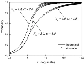
(3) Vol.2015-MPS-104 No.10 2015/7/27. IPSJ SIG Technical Report. t ≥ 0. Pareto Inter-Contact Time: Analysis of real mobility traces and synthetic mobility models suggests that Pareto distribution can well approximate the distribution of intercontact times in OppNets [5]–[7]. Thus, we assume all intercontact times Xi ’s for node u1 and u2 feature a Pareto distribution with scalar parameters xm > 0 and α > 1 as follow [6], [9], { ( )α 1 − xxm if x ≥ xm , FX (x) = P r{X ≤ x} = 0 if 0 < x < xm , (1) from which we also have the mean value αxm . X = E{X} = α−1. (2). III. I NTER -C ONTACT T IME A NALYSIS In this section we derive closed-form results for the distribution of residual inter-contact time. We first present a lemma below, which will be used in our following derivation. Lemma 1. Consider the contact process {N (t); t > 0} between u1 and u2 defined before. Suppose a message arrives at u1 at time t. For given constant a, δ and x satisfying 0 ≤ a < a + δ ≤ t, a + 2δ ≤ x, let E denote the following event e E = {a ≤ A(t) < a + δ, x − δ < X(t) ≤ x},. (3). where A(t) is the age of inter-contact time at time t for that e message, X(t) is the concerned inter-contact time. Then, we have ( )( ) P r{E} = m(t − a) − m(t − a − δ) FX (x) − FX (x − δ) (4) where m(t) = E{N (t)}.. Theorem 2. For an opportunistic network with Pareto intercontact time given in (1), the limiting distribution of residual inter-contact time R(t) of a message as t → ∞ is { ( )α−1 if r ≥ xm , 1 − α1 xrm lim P r{R(t) ≤ r} = rα−r t→∞ if 0 < r < xm . αxm (6) Proof. Due to space limitation, see our report [8] for a complete proof. Finally, we want to find out how long it will take a node with a new arrival message to contact another node in the OppNet, thus having opportunities to forward the message to the next node. Suppose a homogeneous opportunistic network of W nodes, where all nodes move independently and the inter-contact times of every pair of nodes feature the same Pareto distribution given in (1). Let Rij (t) be the residual inter-contact time for node i and node j, then the time interval R∗ (t) from time t the message arrives at node u1 to the time u1 contacts any one of the other W − 1 nodes in the network is { } R∗ (t) = min R12 (t), R13 (t), · · · , R1W (t) (7) Lemma 2. The limiting distribution of R∗ (t) is given as follows. lim P r{R∗ (t) ≤ r} t→∞ { ( )W −1 ( xm )(α−1)(W −1) 1 − α1 = ( αxm −rα+rr)W −1 1− αxm. if r ≥ xm , if 0 < r < xm . (8). Proof. P r{R∗ (t) ≤ r} = 1 − P r{R∗ (t) > r}. (9). Proof. Since the contact process forms a renewal process, this lemma follows directly from Theorem 5.7.2 [11].. =1 − P r{R12 (t) > r, R13 (t) > r, · · · , R1W (t) > r} (10) =1 − P r{R12 (t) > r}P r{R13 (t) > r} · · · P r{R1W (t) > r} (11). Now, we derive the transient distribution of residual intercontact time for nodes u1 and u2 .. where (11) follows from the independence of node mobility. After substituting (6) into (11), we got (8).. Theorem 1. For an OppNet with Pareto inter-contact times given in (1), the transient distribution of residual inter-contact time R(t) for a message at time t is ( x )α ( x )α m m P r{R(t) ≤ r} = − t t+r ∫ t ( ) + FX (t − τ + r) − FX (t − τ ) dm(τ ). IV. S IMULATION R ESULTS. 0. (5) where r > 0. Proof. Due to space limitation, see our report [8] for a complete proof. Next, we derive the limiting distribution of residual intercontact time R(t) as t → ∞.. ⓒ 2015 Information Processing Society of Japan. To validate the derived distribution of residual inter-contact time, we developed a customized simulator in C++ to simulate the contact process between two nodes u1 , u2 , the random message arrival process to node u1 , and observe the residual inter-contact times regarding message arrivals. Specifically, we simulated three different network scenarios where inter-contact times between u1 and u2 all follow Pareto distribution but with different scalar parameter settings: (xm = 1.0, α = 1.5), (xm = 1.0, α = 2.0) and (xm = 2.0, α = 3.0). We assume messages arrive at node u1 according to a Poisson process with arrival rate of 0.001. During simulations, we measured the residual inter-contact time for a message as the time interval from the time it arrives at u1 to the next time u1 contacts u2 . From the measured residual inter-contact times,. 3.

(4) Vol.2015-MPS-104 No.10 2015/7/27. IPSJ SIG Technical Report. we calculated their distribution. The simulated distributions under three network scenarios are presented in Fig.3, where corresponding theoretical distributions are also given for comparison. From Fig.3, we can see that our derived distributions for residual inter-contact time perfectly match the simulated ones, verifying our theoretical results.. 1.0. X. m. = 1.0,. = 2.0. Probability. 0.8. X. m. = 1.0,. = 1.5. 0.6. X. 0.4. m. = 2.0,. = 3.0. theoretical. 0.2. simulation. [5] A. Chaintreau, P. Hui, J. Crowcroft, C. Diot, R. Gass, and J. Scott, “Impact of human mobility on opportunistic forwarding algorithms,” IEEE Transactions on Mobile Computing, vol. 6, no. 6, pp. 606–620, April 2007. [6] T. Karagiannis, J.-Y. L. Boudec, and M. Vojnovic, “Power law and exponential decay of intercontact times between mobile devices,” IEEE Transactions on Mobile Computing, vol. 9, no. 10, pp. 1377–1390, August 2010. [7] H. Cai and D. Y. Eun, “Crossing over the bounded domain: From exponential to power-law intermeeting time in mobile ad hoc networks,” IEEE/ACM Transactions on Networking, vol. 17, no. 5, pp. 1578–1591, October 2009. [8] J. Gao and M. Ito, “Residual inter-contact time for opportunistic networks with pareto inter-contact time: Two nodes case,” NAIST, Tech. Rep., June 2015, [Online]. Available: http://researchplatform.blogspot.jp/. [9] C. Boldrini, M. Conti, and A. Passarella, “From pareto inter-contact times to residuals,” IEEE Communications Letters, vol. 15, no. 11, pp. 1256–1258, November 2011. [10] A. Clauset, C. R. Shalizi, and M. E. J. Newman, “Power-law distributions in empirical data,” SIAM Review, vol. 51, no. 4, pp. 661–703, 2009. [11] R. G. Gallager, Stochastic Processes: Theory for Applications. Cambridge University Press, February 2014. [12] J. Leguay, T. Friedman, and V. Conan, “Evaluating mobility pattern space routing for dtns,” in Proceedings of 25th IEEE International Conference on Computer Communications (INFOCOM), 2006.. 0.0 0.1. 1. 10. r. 100. 1000. (log scale). Fig. 3. Disbribution of residual inter-contact time under different Pareto distribution parameters.. V. C ONCLUSION In this paper, we rigorously derived the distribution of residual inter-contact time for opportunistic networks with Pareto inter-contact times. Our results have important implications for applications (by the law of large numbers): for a homogeneous OppNet, where contacts of all node pairs follow common inter-contact time distribution (e.g., students in a campus and corporate users [12]), the distribution of residual inter-contact times can be found out by collecting samples of residual intercontact times from all node pairs in stead of collecting samples from the same node pair for a long time. This creates great experiment convenience, since long-time tracking of the same pair of nodes is usually prohibited due to privacy while shorttime tracking all node pairs is much easier. R EFERENCES [1] L. Pelusi, A. Passarella, and M. Conti, “Opportunistic networking: Data forwarding in disconnected mobile ad hoc networks,” IEEE Communications Magazine, vol. 44, no. 11, pp. 134–141, November 2006. [2] M. McNett and G. M. Voelker, “Access and mobility of wireless pda users,” ACM SIGMOBILE Mobile Computing and Communications Review, vol. 9, no. 2, pp. 40–55, April 2005. [3] J. Su, A. Chin, A. Popivanova, A. Goel, and E. de Lara, “User mobility for opportunistic ad-hoc networking,” in Proceedings of the Sixth IEEE Workshop on Mobile Computing Systems and Applications (WMCSA), 2004. [4] N. Eagle and A. Pentland, “Reality mining: sensing complex social systems,” Personal and Ubiquitous Computing, vol. 10, no. 4, pp. 255– 268, May 2006.. ⓒ 2015 Information Processing Society of Japan. 4.

(5)