Relationship between Queue-Length and Waiting Time Distributions in a Priority Queue with Batch Arrivals

Journal of the Operations Research Society of Japan

VoJ. 37, No. 1, March 1994

RELATIONSHIP BET'WEEN QUEUE-LENGTH AND WAITING TIME DISRIBUTIONS IN A PRIORITY QUEUE WITH BATCH ARRIVALS

Yoshitaka Takahashi Masakiyo Miyazawa NTT Laboratories Science University of Tokyo

(Received July 9, 1992; Revised March 11, 1993)

Abstract We consider a single-server priority queue with batch arrivals. We treat the head-of-the-line (HL) or preemptive-resume (PR) priority rule. Assuming that the arrival process of batches is renewal for each priority class and using the point process approach, we express the individual class queue-length distribution in terms of the waiting time and the completion time distributions. Assuming further a batch Poisson an-ival for each class, together with the previous result on the Laplace-Stieltjes transforms for the waiting time and completion time distributions, we derive the z-transform for the queue-length distribution in closed fonn.

1. Introduction

We consider a multi-class single-server priority queue with batch arrivals, where the batch interarrival times and the customer service times are respectively independent and identically distributed (i.i.d.) for an individual class. We assume the head-of-the-line (HL) or preemptive-resume (PR) priority rule. We will denote this priority queue by GIX /GI;I (HL or PR); see Section 3 for its detail description. The purpose of this paper is to obtain the individual class queue-length distribution in terms of the waiting time and completion time distributions. Especially for the multi-class batch Poisson arrival M

X

/GI;I

(HL or PR) priority queue, we will obtain the z-transfonn for the individual class queue-length distribution in closed form.

So far, there have been few results on the individual class queue-length distribution for the multi-class batch Poisson arrival priority queue. Indeed, for the two-class

M

X

/GI;I

(HL) priority queue, only Hawkes [8] has obtained the z-transform for the queue-length dish'i-but ion using the supplementary variable approach. It seems difficult to extend this two-class result [8] to the multi-class priority queue, since we have to solve a multi-dimensional func-tional equation. On the other hand, there have been fruitful results on the Laplace-Stieltjes transforms (LSTs) for the individual waiting time and completion time distributions. For the multi-class

1I1X

/GI;I

(HL or PR) priority queue, Takagi and Takahashi [18] have ob-tained these LSTs using the delay-cycle approach without solving such a multi-dimensional equation. However, the delay-cycle approach does not provide us the queue-length informa-tion. See also Chaudhry and Templeton [4], Meister [14], Takahashi and Takagi [20J for this situation.

Consequently, it will be useful if we get a distributional form of Little's law (abbreviated as DFLL) which gives the queue-length distribution in terms of the waiting time distribution,

at least for the multi-class MX

/GI/1

(HL) priority queue. Several previous works on DFLL are worth mentioning. Assuming Poisson arrivals, Keilson and Servi [10,11] have derived a

--DFLL for the two-class M/GI/1 (HL) priority queue [11]. Their approach [10,11] is strongly based on the Poisson arrival assumption, and so it does not straightforwardly apply to a batch Poisson arrival queue. Assuming a renewal arrival FIFO (non-priority) queue and using the sample-path approach, Brumelle [2) has obtained the queue-length moments in terms of the waiting time and the renewal function for the arrival process, and has presented the moment-relationship between the queue-length and waiting time distributions for the Poisson arrival FIFO queue, which refines the result of Haji and Newell [6]. Note that all these previous works have treated single-arrival queue; see also Whitt [22, Section 8]. Only Brandt et al. [1] have presented a DFLL for the MX /GI/l FIFO queue. However, there are

few results on DFLL for batch-arrival priority queues.

This paper is organized as follows. In Section 2, we introduce notations and show a preliminary result from the stationary point process theory. Section 3 is devoted to the observation of the batch-arrival priority queue under the Palm distribution (given that a

class-p batch arrives at the system at time origin). In Section 4, we express the individual class queue-length distribution for the

GJX /Glh

(HL or PR) priority queue in terms of the corresponding class waiting time and completion time distributions. In Section 5, for the M

X IGlh

(HL or PR) priority queue, we obtain the z-transform for the queue-length distribution in closed form, by using the results ill Sections 3 and 4 together with the LSTs for the waiting time and completion time distributions previously obtained by Takagi and Takahashi [18].

2. The muIticlass batch-arrival point processes

Let R be the real space, and Z be the set of all integers, i.e., R== (-00,00), Z== { .. ·,-1,O,1,2, .. ·}.

We consider a probability space (n, F, P) with a time-shift operator group {TS} on n. Here,

{TS} is referred to as a time-shift operator group on

n,

if for each s E R, T S is a measurable mapping from (n, F) to (n, F), and if

TS

0 Tt(w)

=

Ts+t(w) (w E

n;

s, t E R)

where 0 denotes the composite operator, i.e. TSoTt(w) == TS(Tt(w)). Whenever no confusion occurs, we suppress argument wEn as in the literature [6, 23]. For example, instead of the equation above, we use

Assume that P is stationary with respect to {'rS} , i.e.,

(P 0 TS)(B) == P(TS B)

=

P(B) (s E R, BE F), where TS _{B == {TS(w)}

En; wEB}.

We introduce our multi-class batch-arrival process. Let I be the number of classes. For each class p(p

=

1,2" .. ,1), let tp,1l be the n-th batch epoch of class p, and Xp,n be the n-th

50 Y. Takafulshi & M. Miyazawa

batch size (number of customers) of class p. We assume that for each p(p

=

1,2"" ,I),

forms a stationary marked point process with respect to P. Here, the mark of 'lip at tp,n is just the batch size X p,n (n E Z). This stationarity is equivalent to assume

'lip 0 1'5

=

{(tp,n - s, Xp,n) }~~-oo for all s E R.

We number those class-p customers who arrive in the n-th batch as (p, n, i) (i

=

1,2"",

Xp,n)' Let tp,n,i be the arrival epo~h of a customer (p, n, i). Note that tp,n

=

tp,n,; for any

i(1 ~ i ~ Xp,n)' We assume {tl),n}n~-oo satisfies···

<

tp,-l

<

tp,o ~ 0

<

tp,l

<

tp,2

< ....

Let XB

==

X{B} be the indicator function of a set B, and let Np,b[or Np,c] be the point process generated by

{tp,n}t~_oo[or {tp,n,d~r ~~-oo],

i.e.,

+00

Np,b(A)

=

L

X{tp,n E A} (A E B(R)),

n=-oo

+00 xv." +00

Np,c(A) =

L L

X{tp,n,i E A} =

L

Xp,IIX{tp,n E A} (A E B(R)),

11=-00 i=1 n=-oo

where B(R) denotes a Borel field on real space R.

Let E denote the expectation with respect to P. The intensities

are assumed to be finite and positive. Define the probability measures on (0, F) by

(B E .1'), (2.1)

(B E F), (2.2)

where XB 0 TS(w)

==

XB(TSw). The probability measure Pp,b[or Pp,c] is called the Palm

dis-tribution with respect to Np,b[or Np,c]' which represents the conditional probability measure of P given that a class-P batch [or customer] arrives at time origin; see Franken et al. [6].

Let Ep,b be the expectation with respect to Pp,b and let Tp,n the interarrival time of

(n - 1)-th and n-th batches (Tp,1I

==

tp,1l - tp,n-t). Note that in general E[Tp,o]

=I

Ep,b[Tp,o].

Note further that Np,b is a simple point process, i.e., Np,b( {tp,n}) = l(n E Z). An inversion formula for (2.1) has been obtained as

(B E F), (2.3)

see Franken et al. [6], Miyazawa [15, 16, 17]. An inversion formula for (2.2) is similarly obtained, but we will use only (2.3) to develop our arguments.

Lemma 2.1 Consider an I-class batch-arrival process. For a bounded random variable u and any p{p

=

1,2"", I}, we have

E[u]

=

Ap,bEp,b[foTp'l U 0 TSds]. _(2.4)

Moreover, if there exists a process {Z(t)} satisfying that Z(s}

=

uoTS(O

<

s

<

Tp,l)(a.s.Pp,b}

and that, for each s

>

O,X{Tp,l

>

s} and Z{s} are uncorrelated with respect to Ep,b, then f+OO

E[u] = Ap,b

10

Pp,b(Tp,l

>

S}Ep,b[Z(s}]ds. (2.5)

Proof. Equation (2.4) is seen to be valid for any indicator function from {2.3}. Any

non-negative function can be a monotone (non-decreasing) limit of these simple functions. {2.4} then follows from the monotone convergence theorem.

We then have from {2.4} and the property of {Z(t}}[Z(s}

=

u 0 TS{O

<

s

<

Tp,d]'

Since X{Tp,l

>

s} and Z(s} are uncorrelated with respect to Ep,b, we have

Ep,b[X{Tp,l

>

s}Z(s}]

=

Pp,b(Tp,l

>

S}Ep,b[Z(S}]. (2.7)

Substituting (2.7) into (2.6) yields (2.5). 0

Remark 2.2 There is a certain confusion in Lemma 3.1 of Miyazawa [16J. We here make it clear by introducing the process {Z(t)}. 0

3. Key observation for the batch-arrival priority queue

We consider a single-server priority queue with I-class batch arrivals. The priority is assumed to be either preemptive-resume {PR} or head-of-the-line {HL} rule. The PR pri-ority rule permits interruptions of customers during service, and on reentering service an interrupted customer resumes service at the point of interruption; the HL rule does not permit interruptions, so that once service begins on a customer, the customer is served to completion, see e.g. [9, 23J. We assume that a customer with a smaller index has precedence over a customer with a greater index (class 1 is the highest, and class I the lowest).

For each individual class p{p = 1,2", " l), the service is based on the SIRO (Service-In, Random-Order) rule within a batch while it is based on the FIFO (First-In, First-Out) rule between batches. By the SIRO rule, a customer of Xp,1I is randomly selected by the server and all the selected customers of Xp,1I are numbered as {p, n, I}, (p, n, 2},'" ,(p, n, Xp,II); see Section 2. The (p, n, i)-customer will be referred to as the i-th customer of batch Xp,II' and it will also be referred to as the (Xp,1I - i

+

I)-tit youngest customer of Xp,II' For example,

(p, n, I)-customer will be referred to as the firs!; customer and also the Xl',n-th youngest customer, within its belonging batch Xp,II'

52 Y. Takahashi & M. Miyazawa

For any p(l ~ p ~ 1), n E Z and i(l ~ i ~ Xp,n), let Sp,n,i be the service time of a

(p, n, i)-customer. We assume that

<I> _{p -}= {(t _{p,n," p,n,} X S _p,n" 1 S _{p,n, ,} 2 ' .. _,p,n, S X _p,n ) } +00 _n=-oo

forms a stationary marked point process with respect to P. Here, the mark of <I>p at tp,n

is the (Xp,n

+

1) -dimensional vector (Xp,n, Sp,n,l, Sp,n,2,"', Sp,n,Xp.J. This assumption is equivalent to

<I>p 0 TS = {(tp,n - S, Xp,n, Sp,n,l, Sp,n,2,'" , Sp,n,xp,J }~~_oofor all s E R.

We further assume that the batch interarrival sequence {Tp,n}~~_oo' the batch size sequence

{Xp,n}~~-oo, and the service time sequence {Sp,n,i};~r ~~-oo are respectively i.i.d. and mutually independent with respect to Pp,b. Since Sp,O,i 0 TS

=

Sp,O,i, Xp,o 0 TS = Xp,o for 0

<

s

<

Tp,l(a.s.Pp,b), note that the sequences

{Xp,n}~~_oo,

and

{Sp,n,i}~r ~~oo

are respectively i.i.d. and independent of {Tp,n}~~_oo with respect to P. Note also that

Ep,b(Xp,O) = E(Xp,o), and El',b(Sp,O,i) = E(Sp,O,i); see Appendix.

Moreover, we assume that <I>p and <I>q are independent with respect to P for p

#

q(l ~ p, q ~ J), as usual in the literature of priority queues

[9, 23].

This assumption excludes the structured input priority queues treated by Takallashi et al. [20,21]. From now on, our input will be denoted by

Z::~=1

<I>p or

GJX

fill

as in Konig et al.

[13]

and our single-server system by the

GJX

/GljI

(HL or PR) priority queue.

Here are basic notations for a class p(p

=

1,2,···,1) in the Gl

x

fGljl (HL or PR) priority queue.

and

lp(t): the number of customers in the system (queue-length) at time t

qp(t): the number of customers in the waiting room (wait-length) at time t

Wp,b,n: the waiting time of the first customer in the n-th arriving batch.

We use the completion time to study the priority queue as in Jaiswal [9]. Consider a

(p, n, i)-customer and the next class-p customer. Here, the next class-p customer is the one with index (p, n, i

+

1) if i

<

Xp,n, and (p, n

+

1,1) if i

=

Xp,n. The completion time Cp,n,i

of a (p, n, i)-customer is then defined as the time duration of a period that begins at the

instant when the service of a (p, n, i)-customer starts and ends at the instant when the server becomes free to take the next class-p customer. In other words, the completion time Cp,n,i

is the interval between the moment at which a (p, n, i)-customer enters service and the first

moment at which there are no higher class {I, 2, ... , p - I} customers in the system after the service of this (p, n, i)-customer. Note that the completion time C1,n,i for the highest

priority class (p

=

1) equals the service time SI,n,i under both PR and HL priority rules. Note also that the completion time Cp,n,i under the PR rule is identical to that under the

HL rule; see e.g. [21, Theorem 3.4].

The total traffic intensity given by

1 1

P

==

2::

Ap,cE[Sp,n,i]

=

L

Ap,bE[Xp,n]E[Sp,n,;] p=1

is assumed to be less than unity. Then, from the stationarity assumption on <!lp, we can construct for each elass p, the queue-length process lp(t) and the wait-length process qp(t)

which are stationary with respect to P, i.e., the processes {lp(t)} and {qp(t)} respectively satisfy

(p = 1,2"", I). (3.1 ) Moreover, the waiting time sequence of the first Gustomer in a batch {Wp,b,n} and the com-pletion time sequence {Cp,n,;} are stationary with respect to Pp,b. See Franken et al [6] and Miyazawa [15] for the construction of these stationary processes {lp(t)} , {qp(t)} , {Wp,b,n},

and {Cp,n,;}.

Consider an event {lp(s) 2: j} for j 2: 0 and s(O

<

s

<

tp,l) in the queue under the measure Pp,b(P

=

1,2"", I). Namely, we consider the conditional event {lp(s) 2: j}, given that a elass-p batch arrived at the queue at the the origin of time axis. Recalling the definition of {tp,n}~~_oo in Section 2, we note that tp,o

=

0, and tp,1

=

Tp,l(a.s.Pp,b)' For s

<

tp,lo there are no arrivals of batches during (O,s), so that all the customers in the system at time

s arrived at or before time origin. Hence, if we introduce:

Z Sp(j, s)

==

{the j-th youngest class-p customer who arrived during (-00,0] still remains in the system at time s}

we have

(3.2) Let -i(i 2: 0) denote the batch index of the j-th youngest class-p customer among the customers who are in the system at time s, i.e.,

X1,,-i

+

Xp,-i+I

+ ... +

Xp,o

2:i

>

Xp,-i+I

+ ... +

Xp,o. (3.3)

If we set Xp,-i+1

+ ... +

Xp,o = k and Xp,-i = m, it is easily verified from these definitions of i, k, and m, that the j-th youngest customer who arrived during (-00, OJ is just the (j -k}-th youngest customer of its belonging batch Xp,-i. By (3.3) we introduce:

Bp(j, i, k, m)

:=

{k

+

In 2: j

>

k, Xp,-i+1

+ ... +

Xp,o = k and Xp,-i = m}. (3.4)

For convenience' sake we further introduce:

RSp(j, i, k, m, s}

==

{the (j - k }-th youngest customer of Xp,-i still remains

ill the system at time

s}.

(3.5)

I t then follows that

Pp,b{ZSp(j,S)

I

Bp(i,k,m)} = ~),dRSp(j,i,k,m,s)

I

Bp(j,i,k,m)}, (3.6)

and

00 j - I 00

Pp,b{ZSp(j,s)}

=

L L L

Pp,b{RSp(j,i,k,ll/',s)

I

Bp(j,i,k,m)}Pp,b{Bp(j,i,k,m}}.

i=O k=O m=j-k

(3.7) We next consider each conditional probability Pp,b{RSp(j, i, k, m, s}

I

Bp(j, i, k, m)} ap-pearing in (3.7) under the HL or PR priority rule, respectively.

54 Y. Takahashi & M. Miyazawa

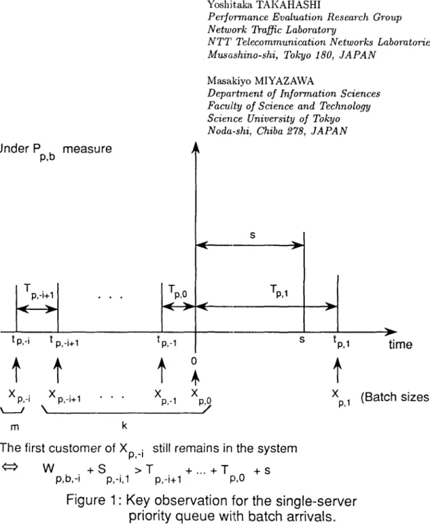
Under the HL rule, a customer in service is not interrupted and the customer departure epoch corresponds to the end of its service time. It then follows that the first [m-th youngest] customer of Xp,-i still remaills in the system at time s, if and only if the sum Wp,-i

+

Sp,-i,l

exceeds Tp,-i+1

+ ... +

Tp,o

+

s; see Figure 1. This follows from the facts that the system sojourn time for the first customer equals 111p,_i

+

Sp,-i,1 and that its sojourn time exceeds

Tp,-i+1

+ ... +

Tp,o

+

s iff the first customer remains in the system at time s. Here, iff denotes if and only if.

In the same way it follows that the second [(m - l)-th youngest] customer of Xp,-i still remains in the system, iff the sum VVp,_i

+

Cp,-i,1

+

Sp,-.,2 exceeds Tp,-i+1

+ ... +

Tp,o

+

s.

The third customer [(m - 2;,-th youngest] of Xp,-i still remains in the system, iff the sum

Wp,-i

+

Cp,-i,l

+

Cp,-i,2

+

S1',-i,3 exceeds Tp,-i+1

+ ... +

7;),0

+

s. Therefore, it follows that the (m - j

+

k

+

l)-th [(j - k)-th youngest] customer of Xp,-i still remains in the system, iff the sum Wp,-i

+

Cp,-i,l

+ ... +

Cp,-i,m-j+k

+

Sp,-;,m-j+k+1 exceeds Tp,-i+1

+ ... +

Tp,o

+

s.

This observation leads to the following equality.

Pp,b{RSp(j, i, k, m, s) IBp(j, i, k, m)}

=: ~),b{Wp,-i

+

Cp,-i,l

+ ... +

Cp,-i,m-Hk

+

Sp,-i,m-Hk+1

>

7;),-i+1

+ ... +

7;),0

+

s} under HL. (3.8) Here, we use the convention for empty sum, e.g. Cp,-i,l

+ ... +

Cp,-i,O = O.

Under the PR priority rule, a customer in service can be interrupted and the customer departure epoch correspond" to the end of its completion time. A similar argument to deriving (3.8) yields that the (j - k)-th youngest customer of Xp,-i still remains in the system, iff the sum of the waiting time of the first customer of the i-th batch (Wp,-i) and m - (j - k)

+

1 completion times (Cp,-i,l

+ ... +

Cp,-i,m-j+k

+

Cp,-i,m-j+k+1) exceeds the time interval Tp,-i+1

+ ... +

Tp,o

+

s, i.e.,

Pp,b{RSp(j,i,k,m,s)

I

Bp(j,i,k,m)}

=

Pp.b{M'p,-i

+

Cp,-i,l

+ ... +

Cp,-i,m-j+k

+

C p,-i,m-Hk+1

>

Tp,-i+1

+ ... +

Tp,o

+

s} under PR. (3.9)

We are in a position to consider an event {qp(s) ~ j} for j ~ 0 and s(O

<

s

<

tp,d. We also introduce:

ZQp(j,s)

==

{the j-th youngest class-p customer who arrived during (-00,0]

still remains in the waiting room at time s};

RQp(j,i,k,m,s)

==

{the (j - k)-th youngest customer of Xp,-i still remains

in the waiting room at time s}.

Regarding the waiting room as the whole system, we have

00 j-1 00 (3.10) (3.11) Pp,b{ZQp(j, s)} =

2: 2: 2:

Pp,b{RQp(j, i, k, m, s)

I

Bp(j, i, k, m)} Pp,b{Bp (j, i, k, m)}. ;=0 k=O m=j-k (3.12)

Under the HL priority rule, the discussions for Pp,b{RSp(j, i, k, m, s)

I

Bp(i, k, m)} can

be applied for Pp,b (RQp(j, i, k, m, s)

I

Bp(j, i, k, m)} to obtain the following equality.

Pp,b{RQp(j, i, k, m, s)

I

Bp(j, i, k, m)} = Pp,i}{Wp,-i

+

Cp,-i,l

+ ... +

Cp,-i,m-(j-k)

>

Tp,-i+l

+ ... +

Tp,o

+

s} under EL. (3.13)

Under the PR rule it is difficult to obtain a similar equation to (3.13) because of the preemptions. However, if we distinguish between the number of customers in the waiting room and that in limbo [21 J (the waiting room :IS used for unserved customers while limbo

is used for interrupted customers), (3.13) is seen to also be valid under PR by the same observation. Henceforth, when considering the PR rule, we will draw this distinction and define the queue-length as the number of customers in the waiting room, so that

Pp,b{RQp(j,i,k,m,s)

I

Bp(j,i,k,m)} = Pp.b{Wp,-i

+

Cp,-i,!

+ ... +

Cp,-i,m-j+k

>

Tp,-i+l

+ ... +

Tp,o

+

s} under PR. (3.14)

We summarize the results obtained above [(2:.2) through (3.14)J in the following lemma.

Lemma 3.1 In a

Gl

x

IGlh

(HL or PR) priority queue, we have for an individual class p

(i) Pp,b{ZSp(j, s)} is given by 00 j - l oc

L L L

Pp,b{vFp,-i

+

Cp,-i,!

+ ... +

Cp,-i,m-j+k

+

Sp,-i,m-j+k+l i=Ok=Om=j-k

>

Tp,-i+1

+ ... +

~),o

+

s}

X Pp,b{Xp,-i+l

+ ... +

Xp,o = k, and Xp,-i = m} under HL,

and

00 j - l 00

L L L

Pp,b{lVp,-i

+

Cp,-i,l

+ ... +

(~),-i,l11-j+k

+

Cp,-i,m-j+k+1 i==O k=O m=j-k

>

Tp,-i+l

+ ... + Tp,o

+

s}

x Pp,b{Xp,-i+l

+ ... +

.Yp,o

=

k, and Xp,-i

=

m} (ii) Pp,b{ZQp(j,s)} is given by

00 j - l 00

under PR.

L L L

Pp,b{Vl't),-i

+

Cp,-i,l

+ ... +

Cp,-i,m-j+k

>

Tp,-i+1

+ ... +

Tp,o

+

s} i=Ok=Om==j-k

x Pp,b{Xp,-i+l

+ ... +

Xp,o = k, and Xp,-i = m} under HL or 1:lR.

4. The queue-length distribution for the Gi'\

IG!';!

(HL or PR) priority queue From the results in Section 3 it follows that ~"l is independent of the event ZSp(j, s) [or ZQp(j, s)J with respect to Pp,b' Indeed, for our

Gj;; IGlh

(HL or PR) priority queue, recall that Tp,l is independent of

{Tp,"}~==_i' {Xp'''}~=

__ i' Wp,-i,

{Sp,-i,"}~~'l;'

and

{Cp,-i,"};;~'l'

for all i

2:

0 with respect to Pp,b. From (3.8) and (:1.9) [or (3.13) and (3.14)J, it is independent

56 Y Takahashi & M. Miyazawa

of the events Bp(j, i, k, m) and RSp(j, i, k, rn, s) [or RQp(j, i, k, rn, s)]. Thus, from (3.7) [or

(3.12)]' we see that Tp,l is independent of ZSp(j, s)[or ZQp(j, s)] with respect to Pp,b.

For an indicator functionu

=

X{lp(O)

2:

j} or X{qp(O)

2:

j}, it follows from (3.1) that

u 0 TS = X{lp(s)

2:

j} or X{q~,(s)

2:

j}. It then follows from (3.2) and (3.10)

u 0 TS

=

X{ZSp(j, s)} or u 0 TS

=

X{ZQp(j, s)} (0

<

s

<

Tp,l) (a.s. Pp,b).

Since Tp,l is independent of the events ZSp(j, s) and ZQp(j, s) as seen above, for each s

>

0 X{Tp,l

>

s} and X{ZSp(j,s)}[or X{ZQp(j,s)}] are uncorrelated with respect to Ep,b'

Namely, both the process {ZSp(j,t)} and {ZQp(j,t)} satisfy the condition for {Z(t)} in Lemma 2.1. Applying Lemma 2.1 with indicator function u = X{lp(O)

2:

j} or X{qp(O)

2:

j},

we obtain the following lemma.

Lemma 4.1 In a

GIX IG!;l

(HL or PR) priority queue, we have for an individual class p

(4.1) and

(4.2)

where lp and qp denote the stationary queue-length and the wait-length, respectively.

To obtain the queue-length and wait-length distributions in terms of the waiting time and completion times, we also need the following lemma.

Lemma 4.2 For a non-negative real-valued random variable Y (with respect to Pp,b) , if

Y is independent of {Tp,-i+1.· .. ,~),a}, we have

(p = 1"", I). (4.3)

Proof. From the definitions of {~},d and Np,b(O, t), we have

1:~

Pp,b(Tp,l

>

S)Pp,b(Y

>

Tp,-i+1

+ ... +

Tp,a

+

s)ds

=

1:~ 1:~

Pp,b(Tp,l

>

S)Pp,b(Y

>

x

+

s)dxPp,b(Tp,-i+1

+ ... +

Tp,() ::; x)ds

[by the stationarity of

{Tp,n}

with respect to ~),bl

1

+00

= u=O Pp,b(Y

>

u)Pp,b(Tp,l

+ ... +

Tp,i ::; U

<

Tp,l

+ .. , +

Tp,i

+

Tp,i+l)du

1

+00

=

u=O Pp,b(Y

>

u)Pp,b(Np,b(O, u) = i)d'a,

which completes the proof. 0

We use the following probability generating functions (pg! s) and Laplace-Stieltjes

trans-forms (LSTs) defined on complex number z or B [lzl ::; 1, Re(B)

>

0) for class p(p =

1,2,'''' I).

Xp(z)

==

Ep,b(z.x:p,n) (pgf for the batch size dilstribution)

and

S;(B)

==

Ep,c(e-·9Sp.n,i) (LST for the service-time distribution)

lp(z)

==

E(zlp(t») (pgf for the stationary queue-length distribution) ftp(z)

==

E(zqp(t)) (pgf for the stationary wait-length distribution)

W;,b(B)

==

Ep,b( e-9Wp ,b,,,) (LST for the stationary waiting-time distribution of a (p, n,

1)-customer)

C;

(B)

==

Ep,b( e--9Cp ,n,;) (LST for the completion time distribution of a (p, n, i)-customer).

We are now in a position to derive the z-transforms of the queue-length and the wait-length distributions. in terms of the completion times as well as the waiting time of the first customer in a batch.

Theorem 4.3 Consider a batch-arrival single-server (Gl

x

jGIj1) priority queue with I

classes. For an individual class p(l ::; p ::; I), we have

_ 1 - z o o m

r+

oo .

lp(z)

=

1 - -z->"p,b

L L

lo Pp,b(Wp,b,O

+

Cp,0,1

+ ... +

Cp,O,I11-j

+

Sp,0,m-j+1

>

s)z1

m=11=1

X Pp,b(Xp,O

=

m)Ep,b(Xp(z)Np,b(O,s»)ds under HL, (4.4)

_ 1 - z o o m

r+

oo .

lp(z)

=

1 - -z->"l',b

L L

lo Pp,b(Wp,b,O

+

(;,0,1

+ ... +

Cp,O,I11-j

+

Cp,0,I11-j+1

>

s)z1

m=11=1

X Pp,b(Xp,O

=

m)Ep,b(_Yp(z)Np.b(O,s»)ds under PR, (4.5)

and

1 - z 00 111

r+oo

.

lJp(z)

=

1 - ~-z->"p,b

L L

lo pp,b(n~o,b,O

+

Cp,0,1

+ ... +

Cp,O,m-j

>

s)z1

111=11=1

X Pp,bCXp,o = m)Ep,b(Xp(z)Np,b(O,s»)ds under HL or PR. (4.6)

Proof. We first prove (4.5) assuming the PR priority rule. It follows from (i) of Lemma 3.1 and (4.1) that

+o()j-1 +00 +00

P(lp 2:: j) = >"p,b

L L L

10

Pp,b(Tp,1

>

s) i=O k=O l11=j-k 0

X Pp,b(Wp,-i

+

Cp,-i,l

+ ... +

C",-i,l11-j+k+1

>

~),-iH

+ ... +

Tp,o

+

s)ds X Pp,b(Xp,-i = m)~),b(Xp,-j+1 -- ...

+

Xp,o = k)

58 Y. Takahashi & M. Miyazaw(l

[by Lemma 4.2]

+00 j - l +00 +00

=

Ap,b

L L L

10

Pp,b(Wp,-i

+

Gp,-i,!

+ ... +

Gp,-i,m-j+Hl

>

s)Pp,b(Np,b(O, s) = i)ds

i=O k=O m=j-k

X Pp,b(Xp,-i = m)Pp,b(Xp,-i+l

+ ... +

Xp,o = k)

+00 j - l +00 +00

=

Ap,b

L L L

10

Pp,b(Wp,O

+

Gp,O,l

+ ... +

Gp,O,m-j+k+l

>

s)Pp,b(Np,b(O, s)

=

i)ds

;=0 k=O m=j-k

X Pp,b(Xp,O = m)Pp,b(Xp,l

+ ... +

Xp,i = k). (4.7)

Here, we used the stationarity of {Wp,n}.{Gp,n,i}. and {Xp,n} with respect to Pp,b.

Multi-plying both sides of (4.7) by zj, summing up with respect to j(j ~ 1), and changing the orders of the summation as

00 00 j - l 00 co 00 00 00 00 00 00 m

LLL L =2::L L L =LL L

L(whereu=j-k),

j=li=Ok=Om=j-k i=Ok=Oj=k+lm=j-k i=Ok=Om=lu=l

we obtain

~

P(lp

~

j)zj = z[l -Zp(z)]

L.J 1 --z

)=1

coo m +00

= Ap,b

I:

L

10

Pp,b(W1},0

+

Gp,Q,l

+ ... +

Gp,Q,m-u+l

>

s)ZU

Ill=l u=l

P (V _ )E (iT ( )Np b(O'S))d

x

p,b ... 1·]J,0 - 1n ]J,b ..'\.p z ' S,

which yields (4.5).

Under the HL priority rule, (4.4) follows if we replace Gp,-i,m-j+k+l by Sp,.-i,m-j-k+l

in the discussion above.

Similarly, (4.6) follows from (ii) of Lemma 3.1 and (4.2). This completes the proof. 0

5. DFLL for the batch Poisson arrival MX

/Glh

(HL or PR) priority queue Let us consider a batch Poisson arrival MX

_/GI/l

_{(HL or PR) priority queue with I}

classes, where the interarrival times of individual class batches are independent, and expo-nentially distributed. For convenience, the set of all customers included a batch is called a

supercustomer. The LST for the service time distribution of a class-p supercustomer is given

by Xp(S;(O)) with mean E[Xp,n]E[Sp,n,;]. Let >';'b be the arrival rate of supercustomers of

class {1,2,··· ,p}, i.e.,

p p

>';'b

=

L

Ak,b =

L

ENk,b[O, 1).

k=l k=l

The LST B\(8) for the service time distribution of a supercustomer of class {1, 2,'" ,p} is then given

by

B:'b(8)

=

>.~

t

>'k,b..'YdSZ(O)). p,b

"'=1

Let

e+

_{p, b}(8) be the LST of the busy period length distribution for supercustomers of class {I, 2""

,plo

It is well known that the LST e;'b(8) satisfies the equation:

If we introduce:

(5.2) the LST C;(O) for the completion time distributiion of a (p, n.i)-customer is obtained as

(5.3) Similarly, the LST C;,b(O) for the completion time distribution of a class-p supercustomer is obtained as

(5.4)

Using the delay-cycle approach as in Kella and Yechiali [12], Takagi et al. [18] and Takahashi et al. [20, 21] have obtained the LST W;,b(O) for the waiting-time distribution of the first customer in a class-p batch as follows:

(5.5) or I * * (1 - p)ap-l

+

L:k=p+l '\k,c(1-Cp(O)) Wp,b(O)

=

0_'\ +,\ C* (0) , p,b p,b p,b (5.6)

in terms of the LS1's for the completion times Cl~(O) and C;,b(O).

We are finally in a position to derive our DFLL (distributional form of Little's law). Note that

(p

=

1,2, ... ,1). (5.7) Note also that for a non-negative real-valued random variable R and a complex number I

with positive real part

lo

+oo P_1J b(R

>

s)e-Sids

=

1 - R*{t)

,

0 ' , (5.8)

where R*(O)

==

ft)"

e-8tdtPp,b(R ::; t).

Let us introduce the following notation for simplicity.

(5.9) Applying Theorem 4.3 leads to the following relationship between the queue-length and the waiting time distributions, which can be regarded as a DFLL.

Theorem 5.1 Consider a hatch Poisson arrival (M

X

/Gl;l) priority queue with I classes. For an individual class p(1 ::; p ::; 1), we have

and 11'(z) = qp(Z)S;(17p) lp( z)

=

qp( z )C; (1]p) under HL, under PR, under HL or PR. (5.10) (5.11) (5.12)

60 Y. Takahashi & M. Miyazawa

Here, TJp is defined by (5.9), Cl~(O) is obtained in (5.3), and Wl~,b(O) in (5.5).

Proof. Substituting (5.7) into (4.6) and using (5.8), we obtain

1 - z o o m

r+

oo .

qp(z) = 1 - -Z-Ap,b

L LlD

Pp,b(Wp,b,O

+

Cp,O,l

+ ... +

CP,O,m-j

>

s)z}

m=l}=l X Pp,b(Xp,O

=

m)Ep,b(Xp(z)Np,b(O, s))ds _ 1 _ 1 - z

~

p (X _ )

~

j 1-W;,b(17p)[C;(TJp)]m-j - L pb pO - m L z -Z m=I" j=l 1 - Xp(z) _ 1 _ [Xp(C;(TJp)) - Xp(z)]

w*

- ( z) (1 _ Xp ( z ) )( C; ( 17p) _ z) p,b ( TJp) ,

which yields (5.12). Equations (5.10) and (5.11) are seen to be valid if we substitute (5.7) into (4.4) or (4.5), respectively. 0

Remark 5.2

a) For a single-class (I = 1) case, (5.10) and (5.11) are reduced to Theorem 7.3.7 in Brandt et a1. [1], where the service interruptions are not allowed.

--b) For a two-class (I

=

2) non-batch arrival (Xp

==

1) M/GI/1 (HL) priority queue, equations (5.10) and (5.12) are reduced to the results in Keilson and Servi [11].

c) So far, we have derived the z-transfonn Ip(z) for the queue-length distribution in terms

of the LST W;,b(O) for the waiting time distributions. The inverse direction obtaining

the LST W;,b(O) in terms of the z-transform Ip(z) is possible if TJp(z) in (5.9) has its

-inverse function. However, for the GI

x

/G!;l (HL or PR) priority queue, the inverse direction is not easy to obtain for lack of the explicit formulas as in Theorem 5.1. 0 Appendix

Consider the probability spaces (0, F, P) and (0, F, Pp,b). If two events Al and A2 are independent with respect to P[or Pp,bj, they are said to be P[or Pp,b]-independent for brevity.

In the following, A is said to be P[or Pp,b]-independent of the batch-arrival process Np,b, if A

is P[or Pp,b]-independent of B for all B E Fp,b where Fp,b is the sub-a-field of F generated

by Np,b, i.e.,

Fp,b

==

a{{Np,b(C)

=

k},k ~

o,e

E B(R)}.

We show the following independence property between P and Pp,b, which is intuitively trivial,

but has not proved yet in the literature. Lemma A.I For any A E F, we have

(a) If A is P-independent of Np,b, then A is Pp,b-independent of Np,b;

(b) If A is Pp,b-independent of Np,b, and if XA 0 TS

=

XA on {s

<

~),t} (a.s .Pp,b), then A is P-independent of Np,b,;

and in these cases,

Proof of (a): The P-independence and the stationarity imply:

Recalling that P(A) is constant and so Fp,b-measurable, and remembering the befinition of

conditional expectation yield

E(XA

°

TS

_I

Fp,b)

=

P(A)_

The definition of the Palm distribution (2_1) then gives for all B E Fp,b:

1 (I

P1),b(AnB) = ~E(lo XAnBOTSNp,b(ds))

p,b 1 (I = ~E(E(lo XAnB

°

TS Np,b(ds)

I

Fp,b)) p,b

=

~E(E(

(I X_4 o TSXB

°

TSNp,b(ds)

I

Fp,b)) "'p,b

10

[from Fp,b - measurability of XB

°

TS] =

~E(

(I E(X_4 () TS

I

Fp,b»W

°

TS Np,b(ds)) "'p,b

10

[by (A_I)]

=

P(A)~E(

(I XB

°

TS Np,b(ds)) "'p,b

10

=

P(A)Pp,b(B)-Taking B as the total event (B = 0), (A_I) is reduced to:

Pp,b(A) = P(A)_

Substituting (A_3) into (A.2), we obtain

Pp,b(A

n

B)

=

P1"b(A)Pp,b(B),

showing that A and Bare Pp,b-independent for all B E

Fp,b-(A_I)

(A_2)

(A_3)

Proof of (b): Note that Pp,b-independence and the additional assumption for XA

°

TS

=

XA

on

{s <

Tp,I} imply:

Ep,b(XA

°

TSX{Tp,,>s}XB)

=

Ep,b(XAX{T",,>s}XB)

=

Pp,b(A)Ep,b(X{Tp,1>S}XB) = Ep,b(Pp,b(A)X{T.,,>s}XB) (for all B E

Fp,b)-Recalling that Pp,b(A)X{T.,,>s} is ~),b- measurable, and remembering the definition of con-ditional expectation yield

Ep,b(XA

°

TS

I

Fp,b)X{T.,,>s}

=

~),b(A)X{T",>s}- (A.4)

The inversion formula (2_3) then gives for all B E Fp,b: (T,,1

P(A

n

B) = Ap,bEl',b(.Io XAnB

°

TSds)

=

Al',bEl',b

(.10

00 X {T.,1 >s} XAnB

°

TS ds ) = Ap,bEl',b(Ep,b(fooo X{Tp,,>s}XAnB

°

TSds

I

Fp,b)) = Al',bEl',b(.fooo Ep,b(XA 0 TS

I

Fp,b)X{Tp,,>s}XB 0 TSds) [by (AA)] =

~J,b(A)Ap,bEp,b(fooo

X{Tp,,>s}XB 0 TSds) = Pp,b(A)P(B)- (A,5)

62 Y. Takahashi & M. Miyazawa

Taking B as the total event n(B

= n),

(A.5) is reduced to (A.3). Substituting (A.3) into (A.5), we obtain

P(A

n

B)

=

P(A)P(B),

which shows that A and Bare P-independent for all BE fp,b. 0

It is clear that Lemma A.l also holds for P and Pp,c, if we replace index (p, b) by (p, c).

Acknowledgements

The authors wish to thank the first referee for his critical and constructive comments. References

[1] A. Brandt, P. Franken and B. Lisek, Stationary Stochastic Models (John Wiley, New

York, 1990).

[2] S. L. Brumelle, A generalization of L

=

,\W to moments of queue length and waiting times, Opemtions Resea1'ch, 20, ll27ll36 (1972).

[3] P. J. Burke, Delays in single-server queues with batch input, Opemtions Research, 23,

830-833 (1975).

[4] M. 1. Chaudhry and J. G. C. Templeton, A First Course in Bulk Queues (John Wiley,

New York, 1983).

[5] R. B. Cooper, Introduct,<:on to Queueing Theory (North-Holland, New York, 1981).

[6] P. Franken, D. Konig, U. Arndt and V. Schmidt, Queues and Point Processes (John Wiley, Chichester, 1982).

[7] R. Haji and G. F. Newell, A relation between stationary queue and waiting distributions, J. Appl. Prob., 8, 617-620 (1971).

[8] A. G. Hawkes, Time dependent solution of a priority queue with bulk arrival, Operations Research, 13, 586-595 (1965).

[9] N. K. Jaiswal, Priority queues (Academic Press, New York, 1968).

[10] J. Keilson and 1. D. Servi, A distributional form of Little's law, Opemtions Research Letters, 7, 223-227 (1988).

[ll] J. Keilson and L. D. Servi, The distributional form of Little's law and the Fuhrmann-Cooper decomposition, Operations Research Letters, 9, 239-247 (1990).

[12] O. Kella and U. Yechiali, Priorities in M/G/1 queue with server vacations, Naval Re-search Logistics, 35, 23-34 (1988).

[13] D. Konig, T. Rolski, V. Schmidt and D. Stoyan, Stochastic processes with imbedded marked point processes (PMP) and their applications in queueing, Math. Operations-forsch. Statist., 9, 125-141 (1978).

[14] B. Meister, Waiting time in a preemptive resume system with compound Poisson input,

Computing, 25, 17--28 (1980).

[15] M. Miyazawa, Time and customer processes in queues with stationary inputs, J. Appl. Prob., 14, 349-357 (197i").

[16] M. Miyazawa, A formal approach to queueing processes in the steady state and their applications, J. Appl. Pmb., 16, 332-346 (1979).

[17] M. Miyazawa, Comparison of the loss probability of the GIx /GI /k queues with a

com-mon traffic intensity, Journal of the Operations Research Society of Japan, 32, 505-516

(1989).

[18] H. Takagi and Y. Takahashi, Priority queues with batch Poisson arrivals, Operations Research Letters, 10, 22;:)-232 (1991).

[19] Y. Takahashi, On the relationship between work load and waiting time in single server queues with hatch input:.;, Opemtions Research Lette1's, 7, 51-56 (1988).

u

[20] Y. Takahashi and H. Takagi, Structured priority queue with batch arrivals, Journal of the Operations Research Society of Japan, :33,242-261 (1990).

[21] Y. Takahashi and S. Shimogawa, Composite priority single-server queue with struetured batch inputs Stochastic Models, 7,481-497 (1991).

[22] W. Whitt, A review of L

=

AW and extensions, Queueing Systems, 9, (1991) 235-268.

[23] R. W. Wolff, Stochastic Modeling and the Theory of Queues (Prentice Hall, New Jersey,

1989).

nder P

b

measure

p, T p,-i+1 Tp,Q

-

"

-

....

...

,

~ " t p,-i _tp,-i+1 t p,-1

t t

t

x .

_p,-I

_{x .}

_p,-I+ 1 X p,-1 II' Yoshitaka TAKAHASHI

Performance Evaluation Resea7'ch Group Network Traffic Laboratory

NTT Telecommunication Networks Laboratories Musashino-shi, Tokyo 180, JAPAN

Masakiyo MIYAZAWA

Department of Information Sciences Faculty of Science and Technology Science University of Tokyo Noda-shi, Chiba 278, JAPAN

s

-

~

'"

, Tp,1

.-

~ ~ , - " , S _{t p,1} ,

ti me

0

t

~

X

x

_{(Batch sizes)}

L - J

\

pJ p,1

m

k

The first customer of

Xp,_i

still remains in the system

<=>

W

+S

>T

+ ... +T

+s

p,b,-i p,-i,1 p,-i+ 1 p,o

Figure 1: Key observation for the single-server

priority queue with batch arrivals.