REVIEW
Fast Statistical Iterative Reconstruction for Mega-voltage
Computed Tomography
Sho Ozaki1, Akihiro Haga2a, Edward Chao3, Calvin Maurer3, Kanabu Nawa1, Takeshi Ohta1, Takahiro Nakamoto1, Yuki Nozawa1, Taiki Magome4, Masahiro Nakano5, and Keiichi Nakagawa1
1Department of Radiology, The University of Tokyo Hospital, Japan, 2Graduate School of Biomedical Science, Tokushima University, Japan, 3Accuray Incorporated. Sunnyvale, CA, US, 4Radiological Science, Komazawa University, Tokyo, Japan, 5Radiation Oncology Department,
Cancer Institute Hospital, Japanese Foundation for Cancer Research, Tokyo, Japan
Abstract : Statistical iterative reconstruction is expected to improve the image quality of computed tomography (CT). However, one of the challenges of iterative reconstruction is its large computational cost. The purpose of this review is to summarize a fast iterative reconstruction algorithm by optimizing reconstruction parameters. Megavolt projection data was acquired from a TomoTherapy system and reconstructed using in-house statistical iterative reconstruction algorithm. Total variation was used as the regularization term and the weight of the regularization term was determined by evaluating signal-to-noise ratio (SNR), contrast-to-noise ratio (CNR), and visual assessment of spatial resolution using Gammex and Cheese phantoms. Gradient decent with an adaptive convergence parameter, ordered subset expectation maximization (OSEM), and CPU/GPU parallelization were applied in order to accelerate the present reconstruction algorithm. The SNR and CNR of the iterative recon-struction were several times better than that of filtered back projection (FBP). The GPU parallelization code combined with the OSEM algorithm reconstructed an image several hundred times faster than a CPU calcula-tion. With 500 iterations, which provided good convergence, our method produced a 512 × 512 pixel image within a few seconds. The image quality of the present algorithm was much better than that of FBP for patient data. J. Med. Invest. 67 : 30-39, February, 2020
Keywords : Statistical iterative reconstruction, Fast reconstruction algorithm, Maximum a posteriori estimation, Megavoltage CT
INTRODUCTION
Helical TomoTherapy (HT) (Accuray, Sunnyvale, CA) is an innovative machine that delivers intensity modulated radiation therapy (IMRT) (1,2), and includes megavoltage (MV) computed tomography (CT) for image guided radiation therapy (IGRT) (3,4). In order to ensure precise image guidance, the image quality of the MVCT is crucial. In particular, detection of soft tissue contrast is very important for soft tissue based registra-tion accuracy and the accuracy of adaptive radiotherapy depends on the accuracy of the soft tissue deformation during the daily treatment (5). However, in general, MVCT images are noisier than that of kilovoltage (kV) CT (4). Furthermore, the relative difference in attenuation coefficients of various soft tissues at MV energies is smaller than at kV energies. The smaller soft tissue attenuation differences lead to smaller contrast differenc-es in MVCT and make it more difficult to register soft tissudifferenc-es accurately.
Statistical iterative reconstruction can improve the image quality of CT without increasing the imaging dose. Unlike con-ventional reconstruction methods such as the filtered back pro-jection (FBP), the iterative reconstruction methods can take into account a priori information including the CT geometry, photon
statistics at the detector, and known properties of the image, in addition to the observed projection data (6). With such knowl-edge-based information, the iterative reconstruction method can reduce noise and improve soft tissue contrast. On the other
hand, a disadvantage of the iterative reconstruction is the large computational cost. Since the method iteratively calculates a reprojection to compare with measured projection data, the total calculation time can be longer. One of the easy ways to reduce the calculation time is to use a GPU-based iterative reconstruc-tion (7-9), where the reconstrucreconstruc-tion time for a set of cone beam CT images with the iterative reconstruction algorithm could be shortened to 77 to 130s (about 100 times faster than with con-ventional approaches). In addition to the GPU parallelization, it is possible to shorten the total calculation time by using the techniques such as an ordered subset expectation maximization (OSEM) algorithm (10). In this review, we summarize an accel-eration method of the statistical iterative reconstruction by using TomoTherapy MVCT system. With utilizing a parallelized CPU/ GPU calculation, we applied several acceleration techniques including an adaptive convergence parameter for the gradient decent method and the OSEM algorithm. The performance and the quality of the reconstructed images of the respective methods were evaluated using phantom and patient data.
ETHICAL STATEMENT
The study was ethically approved by the institutional review board at the University of Tokyo Hospital (reference number 3372). Written informed consent was obtained from all patients whose data were used in this study.
MATERIALS AND METHODS
Iterative reconstruction scheme
In this section, we briefly explain the basics of the statistical iterative CT reconstruction. In this study, the maximum a
poste-The Journal of Medical Investigation Vol. 67 2020
Received for publication November 27, 2019 ; accepted December 24, 2019.
Address correspondence and reprint requests to Akihiro Haga, PhD, 3-18-15 Kuramoto, Tokushima 770-8503, Japan and Fax : +81-88-633-9024.
riori (MAP) approach was employed as the image reconstruction
framework (11-14). The concept of the MAP approach is to max-imize the posteriori probability of reconstruction images with observed projection (or sinogram) data and a prior information about the image, encoded in the regularization term. Recon-structed images can be obtained from an iterative process to maximize the log a posteriori probability function ln p(μ*|y) as,
μ* = μ* ln p(μ*|y) subject to μ* > 0, (1)
where
ln p(μ*|y) ~ ln p(y|μ*) +ln p(μ*) = L(μ*) + αR(μ*) . (2)
Here L(μ*) = ln p(y|μ*) expresses the log-likelihood
probabil-ity function of observing the projection data set y at the given
expectation of the image μ*, whereas αR(μ*) = ln p(μ*) stands
for the regularization term in the optimization process with a hyper parameter α controlling the weight of the regularization. We assumed that the photon statistics at the detector obeys the Poisson distribution and employed the total variation (TV) as the regularization term. The TV term penalizes a large difference between the image values of a certain position and its neighbors, and thus reduces the noise of the image. At the same time, how-ever, this term also reduces the sharpness of object edges in the image, which leads to edge blurring. Therefore, in general, the noise reduction must be balanced against the negative impact of edge blurring. We seek the appropriate value of the weight α by examining the trade-off.
In the optimization of Eq. (1), the gradient decent method in-cluding the parameter adaptation was employed,
∂
μr*(n+1) = μr*(n)+ λ(n)——— (L(μ*) + αR(μ*)), (3) ∂μr*(n)
where n is the number of the iteration step, and r means the
index of the pixel to be reconstructed. λ(n) is the parameter which is adjusted to accelerate the calculation iteration step by iteration step as described in the following. It is noted that, as well as the value of λ(n), the initial image setting μ
r*(0) can affect the conver-gence speed.
Data acquisition and Computer used in reconstruction
Gammex phantom (Gammex, Middleton, WI) and Cheese phantom (Accuray, Sunnyvale, CA) were used in the analysis as well as the two patients for visual demonstration.
The reconstruction size of the image is 512×512 with an equal pixel size of 1mm for the one slice. The CPU/GPU specs in the computer used in this study (HP customized workstation : Z840/ Z800) are shown as follows :
CPU : Xeon(R) X5690 (×2 : 12 threads) / Xeon(R) E5-2687Wv (×2 : 20 threads)
GPU : GeForce GTX 1080 Ti Parameter optimization
The weight of the TV regularization term α was set as 0, 0.0001, 0.0002, and 0.0003. The optimal values of the weight pa-rameter were determined by estimating the signal-to-noise ratio (SNR), the contrast-to-noise ratio (CNR), the visual resolution, and the edge blurring effect. For SNR/CNR and edge blurring analyses, the Gammex phantom was used, whereas for visual resolution, the Cheese phantom was used. The region-of-inter-ests (ROIs) used in the SNR/CNR analysis as well as their defi-nitions and the edge blurring analysis method are mentioned in the supplemental material.
Although a relatively large value of λ(n) in Eq. (3) gives a rapid convergence, a too large value leads to non-convergence. Also the best value could depend on the iteration step. Therefore, we employed the following adaptive convergence parameter which depends on the iteration step : when the objective function being the square of difference between a reprojection and a projection decreases, the convergence parameter is increased as
λ(n+1) = λ(n) + 0.0001. (4)
When the objective function increases, the parameter is de-creased as
λ(n+1) = λ(n) - 0.0002. (5)
The initial value of this parameter was set as 0.01. As men-tioned, the initial image setting μr*(0) can also affect the conver-gence speed. In this study, homogeneous images with μr*(0) =0, 0.05, and 0.1 [cm-1] were tested.
Ordered subset expectation maximization and Parallel computing The ordered subset expectation maximization (OSEM) is a well-known method to accelerate the convergence of the iterative reconstruction algorithm (10). A basic idea of OSEM is to divide the original projection data into a subset of the data and to use the different subset in each iteration step. The easiest way to di-vide the projection data into subset is to thin the sinogram height out. In the HT system, the data sampling time is 80 Hz, and it takes 10 sec for one rotation. Hence the sinogram height is 800. We thinned the sinogram height out by 1/2, 1/5, 1/10, 1/20, and 1/40 (defined as the thinning parameter) with an equal interval (the sinogram height used in each iteration step is 400, 160, 80, 40, and 20, respectively). For instance, in the 1/40 case, 40 iterations are needed to cover the whole sinogram data, so that the convergence could be relatively slow. Therefore, the conver-gence as well as its efficiency has to be verified carefully. Here, it should be noted that the regularization weight α in the OSEM method is multiplied by the thinning parameter in order to keep the ratio of log-likelihood function with regularization term.
For the parallel computing, we applied openMP for CPU parallelization, and cuda for GPU parallelization. In the next section, the reconstruction speeds with the several cases of the number of thinning out for OSEM described above will be compared.
RESULT AND DISCUSSION
Total variation parameter
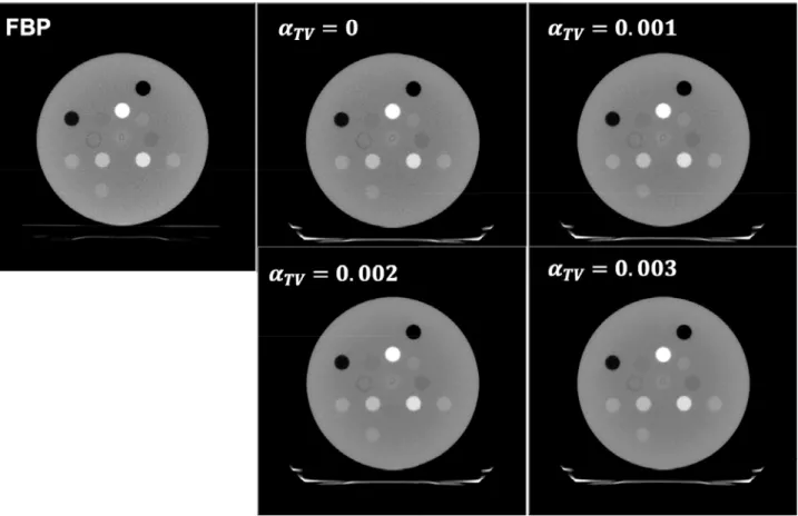
In order to determine the total variation parameter, the SNR and the CNR in the eleven insertions of the Gammex phantom were analyzed (see Fig. S-2 in the supplemental material for the reconstructed images). Figure 1 shows the results of the SNR and the CNR. In these results, the SNR and the CNR of the iterative reconstruction are normalized by the values of the FBP. In Fig. 1, both of the SNR and the CNR converge as the iteration number increases, and their values with the finite α are always larger than that of the FBP image. On the other hand, as mentioned above, noise suppression is generally accom-panied by a trade-off of reduced image sharpness. This is seen in Fig. 2, where we can see that as the total variation parameter increases, the noise of the image decreases but the visibility of the small holes in the resolution plug of the cheese phantom also decreases. From these results, we concluded that 0.0001 < α < 0.0002 maintains acceptable image resolution while achieving significant noise suppression.
Convergence parameter and initial image setting
Figure 3 shows the square of difference of the observed pro-jection and the repropro-jection evaluated from the reconstructed image for a variety of parameters, where convergence is charac-terized by the square of the difference between a projection and a reprojection in the sinogram domain. As expected, better con-vergence is obtained with the adaptive concon-vergence parameter method. With the adaptive convergence method, a similar degree of convergence is achieved with 500 iterations compared to 1500 iterations using a constant convergence parameter. It should be
Fig 1. Signal-to-noise ratio (SNR) and contrast-to-noise ratio (CNR)
Fig 2. Visual assessment for spatial resolutions (Cheese phantom).
Fig 3. Square of difference of the observed projection and the reprojection evaluated from the reconstruct-ed image as a function of the number of iterations.
noted that the oscillation of the square difference is also caused by this adaptation ; As the convergence parameter becomes gradually large according to the Eq. (4), the images grow away from the optimal values. Eventually, the square difference turns to increase and numerically diverge. This increasing behavior is however suppressed by decreasing the parameter as Eq. (5) when the square difference is increased. Due to this oscillation, we employed the reconstructed image at the minimum of the oscillation of the square difference.
The initial homogeneous images were set to values of 0, 0.05 and 0.1 [cm-1], and the best convergence was obtained for 0.05 [cm-1] in the Gammex phantom, though the difference was so small. This was an expected result because the reconstructed value of μ* in the water area was approximately 0.07 [cm-1] and the mean value of the reconstructed image including the air area was 0.026 [cm-1]. Other two phantoms with the different radius also gave the same result (see Table S-1 in supplemental file).
It was found that the adaptive convergence parameter and the initial image setting accelerated the convergence approximately three times faster than that with the constant convergence pa-rameter starting with the “zero” image.
CPU parallelization and OSEM method
The convergence with applying the OSEM method is also shown in Fig. 3, where the oscillation is emphasized. The con-vergence needs relatively larger iteration steps in the OSEM method, because the reconstructed image and its reprojection are obtained from thinned-out projection data. However, this apparent disadvantage is overcome by large reduction of the calculation time for the one iteration, thanks to the thinning. Eventually, the OSEM method highly accelerates the recon-struction speed.
We found that 500 iterations were an enough number of itera-tion in which the square of difference converges in the case of the thinning parameter more than 1/20, whereas more iterations was required in the thinning parameter of 1/40. Combining OSEM with CPU parallelization yielded the image reconstruc-tion time more than 40 times faster than the original single CPU implementation, and more than 8 times faster than the CPU parallelization without OSEM. Consequently, combining the OSEM with CPU parallelization considerably accelerates the calculation.
GPU computing
In our reconstruction algorithm, the reprojection and the estimation processes occupy a large fraction of the calculation time. Therefore, we coded these parts of the reconstruction using CUDA GPU processing. Table 1 shows the average calculation time for reconstructing one image slice. Although the results depend on the iteration number and OSEM parameter, the GPU code produces an image more than 10 times faster than the par-allelized CPU code without degrading image quality. Using the GPU code, a high quality image can be reconstructed at a speed of 3.71 seconds per slice. This large improvement in iterative reconstruction speed on the GPU is achieved without any deg-radation in image quality compared to the CPU reconstructed images.
Reconstructed images
Finally, the representative reconstructed images with α = 0.0002 are shown in Fig. 4. For comparison, FBP reconstruction images are also shown there. In addition to the noise reduction seen in Figs. 4(a)-4(b), a relatively large reconstructed region (field of view) was achieved with the iterative reconstruction approach seen in Figs. 4(c)-(d). Owing to the fan beam geometry, information of the projection data decrease at a fringe region of FOV. Therefore, FBP fails to reconstruct the image at the edge of the body (Fig. 4-(c)). On the other hand, the statistical iterative reconstruction algorithm can reconstruct the image with a fewer projection data (the examination of the reconstruction using a half of projection data is given in supplemental file), and thus shows much better image quality at the edge (Fig. 4-(d)). From these image quality improvements, it can be said that we can clinically use the iterative reconstruction algorithm for MVCT.
CONCLUSION
We investigated the clinical feasibility of a statistical iterative reconstruction method by using MVCT on a HT system. An image from the iterative reconstruction can be obtained within few seconds per image slice with a size of 512 × 512. In addition, the image quality of the iterative method is much better than that of the FBP. It can be concluded that the iterative recon-Table 1. Reconstruction speed [s] per one slice image with 512×512.
Thinning parameter 1 1/2 1/5 1/10 1/20 1/40
CPU (12 threads) 442.91 244.34 138.77 80.68 58.79 43.29
CPU (20 threads) 325.40 191.16 94.40 51.21 35.99 24.59
GPU (GTX1080Ti) 11.00 7.76 5.37 4.30 3.71 3.39
Fig 4. Reconstructed images : (a) head region using filtered back projection, (b) head region using iterative reconstruction, (c) abdom-inal region using filtered back projection, and (d) abdomabdom-inal region using iterative reconstruction.
struction with GPU is fast enough for clinical use, and largely improves the CT images. The present review focused on the MVCT because the impact of the iterative reconstruction was enhanced in its relatively poor quality of images. However, the present algorithm can be cooperated with all of reconstruction algorithms for kVCT, CBCT, and dual energy CT and the appli-cation of the fast statistical iterative reconstruction is expected more and more.
COMPETING INTERESTS
Edward Chao and Calvin Maurer are officers of Accuray Inc. Keiichi Nakagawa had a research grant from Accuray Inc (between Jan. 2018 and Dec. 2018).
ACKNOWLEDGEMENTS
This study was partially supported by a Grant-in-Aid from JSPS (Japan Society for the Promotion of Science) KAKENHI JP Scientific Research (C) Grant Number 15K08691.
REFERENCES
1. Mackie TR, Homes T, Swerdloff S, Reckwerdt P, Deasy JO, Yang J, Paliwal B, Kinsella T : Tomotherapy : A new concept for the delivery of dynamic conformal radiotherapy. Med. Phys 20 : 1709-1719, 1993
2. Mackie TR : History of tomotherapy. Phys. Med. Biol 51 : R427-R453, 2006
3. Meeks SL, Harmon JF Jr, Langen KM, Willoughby TR, Wagner TH, Kupelian PA : Performance characterization of magavoltage computed tomography imaging on a helical tomotherapy unit. Med. phys 32 : 2673-2681, 2005
4. Ruchala KJ, Olivera GH, Schloesser EA, Mackie TR :
Megavoltage CT on a tomotherapy system. Phys. Med. Biol 44 : 2597-2621, 1999
5. Langen K, Meeks S, Poole D, Wagner TH, Willoughby TR, Kupelian PA, Ruchala KJ, Haimerl J, Olivera GH : The use of megavoltage CT (MVCT) images for dose recomputations. Phys. Med. Biol 50 : 4259, 2005
6. Nassi M, Brody WR, Medoff BP, Macovski A : Iterative Reconstruction-Reprojection : An Algorithm for Limited Data Cardiac-Computed Tomography, IEEE Trans. Med. Imaging 9 : 333 - 341, 1982
7. Scherl H, Keck B, Kowarschik M, Hornegger J : Fast GPU-Based CT Reconstruction using the Common Unified Device Architecture (CUDA). IEEE Nuclear Science Sym-posium Conference Record : M26-280, 2017
8. Jia X, Lou Y, Li R, Song WY, Jiang S : GPU-based fast cone beam CT reconstruction from undersampled and noisy projection data via total variation. Med. Phys 37 : 1757-1760, 2010
9. Xu Q, Yang D, Tan J, Anastasio M : Total variation (TV) based fast convergent iterative CBCT reconstruction with GPU acceleration. Med. Phys 39 : 3857, 2012
10. Hudson HM, Larkin R : Accelerated image reconstruction using ordered subsets of projection data. IEEE Trans. Med. Imaging 13 : 601-609, 2014
11. Tang J, Nett BE, Chen GH : Performance comparison be-tween total variation (TV)-based compressed sensing and statistical iterative reconstruction algorithms. Phys. Med. Biol 54 : 5781-5804, 2009
12. Hanson KM, Wecksung GW : Bayesian approach to limit-ed-angle reconstruction in computed tomography. J. Opt. Soc. Am 73 : 1501, 1983
13. Green PJ : Bayesian reconstructions from emission tomog-raphy data using a modified EM algorithm. IEEE Trans. Med. Imaging 9 : 84-93, 1990
14. Lange K, Fessler J : Globally convergent algorithms for maximum a posteriori transmission tomography. IEEE Trans. Image Process 4 : 1430-1438, 1995
Supplemental material (Fast Statistical Iterative
Re-construction for Mega-voltage Computed Tomography)
I. NOTE 1 : REGIONS ANALYZED IN SIGNAL-TO-NOISE RATIO (SNR) AND CONTRAST-TO-NOISE RATIO (CNR)
The regions analyzed in signal-to-noise ratio (SNR) and con-trast-to-noise ratio (CNR) are indicated in Fig. S-1, where the Gammex phantom was used with 12 materials (the solid water regions ⑤〜⑧ as well as water region ⑨ were removed in the analysis). The SNR and CNR are defined as,
=; =;
where MROI and ROI are the mean and the standard deviation of signal values inside the ROI, respectively.
Fig. S-2 shows the images reconstructed by the statistical it-erative reconstruction method with several values of the weight parameter α. For the comparison, the result from FBP is also shown.
II. NOTE 2 : EDGE BLURRING ANALYSIS
The SNR and the CNR with the finite total variation parame-ter, αTV, are always larger than that of the filtered back projection
(FBP) image as shown in Fig. 1 in the Technical Note. However, the noise suppression generally accompanies the trade-off re-lation with the blurring. The visual evaluation was performed with the cheese phantom as described in the Technical Note. In addition, the quantitative evaluation of the blurring effect in our statistical iterative reconstruction was performed with the high density circular object in Gammex phantom by its penumbra analysis. The line profiles at the same location (the red dotted line in the upper-left panel in Fig. S-3) were obtained in each iteration step, and fitted by a sigmoid function. Then, the pen-umbra width defined by the width between 20-80% values of the profile was evaluated. The lower panel in Fig. S-3 shows the re-sult of the penumbra width as a function of the iteration number. As the iteration number was increased, the penumbra width was narrower. We found that the penumbra width is not so sensitive to the change of the total variation parameter.
III. NOTE 3: CALCULATION TIME
The calculation time of our statistical iterative reconstruction with a single CPU and a xed convergence parameter (λ = 0.001) was 5,037.9 [s] for 1,000 iterations in 512 × 512 image. This was reduced to 946.2 [s] by OPEN MP parallel processing with 20 threads (the efficiency ratio was 5.3).
The efficiency of the adaptive convergence parameter depends on the reconstructed images; A number of the iterations required to produce the Mahalanobis’ distance between the sinogram and the forward projection, which is the same value as that obtained
Fig. S-3 : Edge blurring analysis.
Fig. S-2 : Reconstructed images. αTV is the weight of the total variation in our statistical iterative reconstruction parameter. The reconstructed images just after 1,000 iterations are selected.
from the 1,000 iterations with a fixed convergence parameter, was shown in Table S-1 with several phantoms. The best effi-ciency was seen in the Gammex phantom whereas the worst efficiency was seen in the Catphan phantom. The Gammex phantom was larger than the Catphan phantom, and it presum-ably affects the convergence speed. The initial image setting was also shown in Table S-1. The efficiency was slightly better in use of the μr*(0) = 0.05. The efficiency in the Catphan phantom was more improved than that in the Gammex phantom, due to the larger air region in the Catphan phantom.
IV. NOTE 4: USING A HALF OF PROJECTION DATA
The statistical iterative reconstruction can reconstruct the image from a fewer projection data. The prior information (in this study, total variation term) plays an important role in data missing area in the reconstruction image. Figure S-4 shows the effect of the reduction of the projection data. The noise is in-creased in the FBP algorithm, whereas the SNR is almost kept, even if the number of projection data is reduced in the statistical iterative reconstruction. This effect can also be seen in the pe-ripheral reconstructed area, especially, with a large body (see Figs. S-5 and S-6).
V. NOTE 5: RECONSTRUCTED IMAGES
Figures S-5 〜 S-10 shows the comparison between FBP and our statistical iterative reconstruction with αTV = 0.002.
Table S-1 : Iteration numbers with same Mahalanobis’ distance as that of the 1,000 iterations with a fixed convergence parameter.
Phantom μr*(0) = 0.1 μr*(0) = 0.05
Gammex 471 448
Cheese 540 512
Catphan 613 543
Fig. S-5 : Reconstructed images for lung region.
Fig. S-6 : Enlarged figures of S-5.
Fig. S-8 : Enlarged gures of S-7.
Fig. S-9 : Reconstructed images for head region.

![Table 1. Reconstruction speed [s] per one slice image with 512 × 512.](https://thumb-ap.123doks.com/thumbv2/123deta/6794882.1165001/4.892.458.811.426.777/table-reconstruction-speed-s-slice-image.webp)