Vol. 64, No. 2, April 2021, pp. 109–127
GENERATING DECISION SUPPORT INFORMATION FOR NURSE SCHEDULING INCLUDING
EFFECTIVE MODIFICATIONS OF SOLUTIONS
Masaya Hasebe Koji Nonobe Wei Wu
Seikei University Hosei University Shizuoka University
Naoaki Katoh Takahito Tanabe Atsuko Ikegami
Seikei University NTT DATA Mathematical Systems Inc. Seikei University
(Received December 11, 2019; Revised November 16, 2020)
Abstract When dealing with real-world problems, optimization models generally include only important structures and omit latent considerations that cannot be practically specified in advance. Therefore, it can be useful for optimization approaches to provide a “solution space” or “many solutions” containing a solution that the decision-maker is likely to accept. The nurse scheduling problem is an important problem in hospitals to maintain their quality of health care. Nowadays, given an instance, mathematical models can be applied to find optimal or near-optimal schedules within realistic computational times. However, even with the help of modern mathematical optimization systems, decision-makers must confirm the quality of obtained solutions and need to manually modify them into an acceptable form. Therefore, general optimization algorithms that provide insufficient information for effective modifications remain impractical for use in many hospitals in Japan.
To improve this situation, we propose a method for a pattern-based formulation to generate information helpful in most practical cases in hospitals and other care facilities in Japan. This approach involves generating many optimal solutions and analyzing their features. Computational results show that the proposed approach provides useful information within a reasonable computational time.
Keywords: Mathematical modeling, decision support information, nurse scheduling,
generation of optimal solutions, network representation
1. Introduction
When dealing with real-world problems, optimization models generally involve only im-portant structures and omit latent considerations that cannot be practically specified in advance. Therefore, it can be useful for optimization approaches to provide a “solution space” or “many solutions,” including a solution that the decision-maker is likely to accept. An important task in hospitals is to schedule nurses so that the quality of health care is maintained at the required level. This must be done while paying attention to many factors simultaneously such as the number and skill level of nurses in each shift, the workload bal-ance of nurses, and their preferences. This is called the nurse scheduling problem (NSP) and is a form of optimization problem in mathematical programming research. Decision-makers must confirm the quality of the schedule even when an optimal solution is obtained from a mathematical model, and they need to further modify the schedule manually according to any additional considerations. This paper focuses on NSPs involving latent (additional) constraints and evaluations that cannot be specified in advance.
The classical NSP has been investigated in many papers, particularly since the late 1990s. There are various definitions of the NSP, reflecting different hospital situations. The NSP is
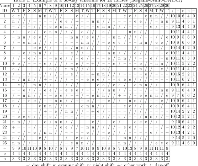
Table 1: Example of a 30-day schedule for 25 nurses (Ikegami-3shift-DATA1) Nurse 1 2 3 4 5 6 7 8 9 10 11 12 13 14 15 16 17 18 19 20 21 22 23 24 25 26 27 28 29 30 ID W T F S S M T W T F S S M T W T F S S M T W T F S S M T W T / – e n + 1 e e / – – n n / / / – – e / / – – / – – – e e / – e n n / / 10 10 6 4 0 2 n / / / – – – – / e e / + – – n n / / – – – – e e / / – n n 9 11 4 5 1 3 – / – – / / – e e n n / / – – – e n n / / / – – – – e / – – 9 13 4 4 0 4 / – – e / – e n n / / / – e / / – e / + – – n n / / – – – – 10 11 4 4 1 5 – n n / e e / – – – – n n / e e / – – n n / / / / – – / / e 10 9 5 6 0 6 / – e n n / / / – – / – – n n / / – e e e / – – n n / e e / 10 8 6 6 0 7 / – – – e e / / – – e / n n / / – – / / – – – / – – – e / – 10 14 4 2 0 8 – – e / n n / / – + – e / / – – / – n n / / – e / / – – – e 10 11 4 4 1 9 / / – e / – – – e e / / – e / – – – e / n n / / – – e / – n 10 11 6 3 0 10 + e / – – – e / / / / – e / – + / – – e / – – – e / – n n / 10 11 5 2 2 11 e / – – – / – e / – n n / / / + – e / – – – – n n / / – e / 10 11 4 4 1 12 / – – / – – / / / – – e / – – + n n / / / – – – – e / – – – 10 15 2 2 1 13 – / n n / / + – / / / – – – e e e / – – e e e / / / – – – – 10 11 6 2 1 14 – e / – n n / / – + / / / – – – e e / e e / – e n n / / – – 10 9 6 4 1 15 – – e / / – e e / – e e e / – – / / n n / / – – – / – – n n 9 11 6 4 0 16 / – n n / / – – e e / – + / – e n n / / + – / – e e n n / e 9 7 6 6 2 17 e / – e e / – – n n / / + – e / – – e / / – n n / / – – e / 10 9 6 4 1 18 / / – – – e n n / / / – – e n n / / – + – e e / / – e e / – 10 9 6 4 1 19 – / – – – / + – e / n n / / – + e / – – – – / / / / – – – – 10 14 2 2 2 20 – e e e / / – e / – – – / – – – – / / – e / – – / n n / / + 10 12 5 2 1 21 n n / / – – e / n n / / – – – e / – – e / – – e e e / / – + 9 10 6 4 1 22 + – – – / – – – / e e / / – n n / / / / – e e / – – – – / + 10 12 4 2 2 23 – – / – e / n n / / – – – – e / / – e / / / – – – – e / – + 10 13 4 2 1 24 e / / – – e / – – – / – e e / – – e / – – n n / / / – – – – 9 14 5 2 0 25 n n / / – – / – – / – e n n / / – – – – n n / / – – / e e e 9 11 4 6 0 – 9 9 10 11 10 9 8 10 7 8 7 9 7 10 11 8 9 10 8 8 9 10 13 8 9 8 11 11 11 9 e 4 4 4 4 4 4 4 4 4 4 4 4 4 4 4 4 4 4 4 4 4 4 4 4 4 4 4 4 4 4 n 3 3 3 3 3 3 3 3 3 3 3 3 3 3 3 3 3 3 3 3 3 3 3 3 3 3 3 3 3 3
–: day shift; e: evening shift; n: night shift; +: other work; /: day-off
usually modeled mathematically as a combinatorial optimization problem. It is known that the NSP is NP-hard [7], and it is difficult to solve in practical applications, even when only relatively few nurses (e.g., fewer than 30) are to be scheduled. Table 1 shows an example of a 30-day schedule for 25 nurses in a three-shift system. This is an optimal solution to the NSP benchmark instance entitled Ikegami-3shift-DATA1 [12], which is available at a benchmark site ([8]). In Table 1, the first and second rows are dates and days of the week, respectively. The 25 nurses, whose IDs are given in the first column, are grouped according to their skill levels and the patients in their charge. Each regular row represents the individual schedule of a specific nurse, where “–,” “e,” “n,” “+,” and “/” stand for “day shift,” “evening shift,” “night shift,” “other work” (typically attending seminars or meetings), and “day-off,” respectively. Table 1 shows the total number of nurses working during each shift for each day. For each nurse, the required total number of days to work on each type of shift is also given.
In this problem, as in most other NSPs, we must consider both shift constraints and nurse constraints. Shift constraints are introduced to maintain a certain level of nursing quality on each shift and to impose lower and upper bounds on the number of nurses working on each shift per day. Nurse constraints control nurse workloads by considering the total number of each shift type that a nurse works, the nurse’s preferences, and sequences of
shifts on consecutive days. We categorize constraints into these categories to be conscious of differences in properties and how to deal with them, but “hard and soft constraint” categorizations that most nurse scheduling models apply [3] are useful as well, as described more precisely in Section 2.
As shown by literature surveys [5, 9, 18], over the past two decades many papers have been published concerning algorithms for the NSP. A number of NSP benchmark instances, including Ikegami-3shift-DATA1, are now available and many researchers have tackled these datasets. In recent real-world case studies, Adoly et al. [1] proposed a formulation based on the idea of a multi-commodity network flow model and applied it to an actual case study in an Egyptian hospital. Hamid et al. [10] proposed a multi-objective mathematical model for the NSP with the hybrid data envelopment analysis (DEA) and augmented ϵ-constraint method, and provided a case study from Iran with 22 nurses and a one-week planning horizon. Zanda et al. [19] showed the applicability of their decision support system based on integer linear programming through a case study in an Italian hospital. Consequently, with progress in computer hardware as well as algorithms, it is now possible to find optimal or nearly optimal schedules in realistic computational times. Thus, once the NSP is modeled as an optimization problem, a sufficiently good schedule can be found.
Even so, in most hospitals in Japan at least, those in charge of nurse scheduling (typically head nurses) still make schedules manually every month, sometimes with the assistance of some form of scheduling software. This is likely because decision support systems do not consider all the necessary constraints, and therefore generate unacceptable schedules, or make schedule editing difficult. Furthermore, creating flexible NSP models would be difficult due to differences in constraints among hospitals. Doing so is not impossible, but in practice it requires a large amount of work to provide a common model and valid parameters.
Stochastic programming [6] and fuzzy programming [15] have been considered as meth-ods for treating uncertainties in real-world NSP applications. Both of these methmeth-ods aim to provide more flexible solutions, but neither can provide human schedulers with additional information when manual modifications are required.
In nurse scheduling, many factors must be simultaneously considered to obtain a satis-factory and usable schedule. Factors such as nurse preferences, personalities, and general health are often difficult to practically specify in advance; sometimes these are latent char-acteristics, and thus are not completely reflected in the mathematical model. It is therefore unrealistic to define an ideal schedule explicitly. Even if such a definition were possible, the amount of work required for the input of such detailed data would be huge. This may cause human schedulers (i.e., decision-makers) to reject an algorithmically produced, math-ematically optimal schedule. Because, it does not comply with constraints (for example, constraints concerning sudden changes in physical condition or interpersonal relationships) derived from the above-mentioned factors that are difficult to specify in advance. This is a long-standing issue that has been discussed in previous studies [11, 14]. Thus, human schedulers often need to make some manual modifications to the schedule for its actual use. As mentioned in [12], the effort required for modifying schedules is known to be reduced when one chooses a schedule that complies with nurse constraints as a starting point for modifications, and then manually relaxes nurse constraints to satisfy shift constraints to the extent possible. This is because the constraints imply the above-mentioned latent factors that only human schedulers can deal with.
To make mathematical optimization techniques effective for human schedulers, there is need for additional information corresponding to an obtained solution, such as whether it is the only optimal solution, whether similar solutions exist, and what parts can be modified.
Our hope is that such additional information can help to further create schedules that reflect potential requirements by modifying the resulting optimal or good solutions.
One common approach to overcoming this difficulty is use of an optimization algorithm that generates provisional schedules for later modification by schedulers. In this approach, in addition to a powerful algorithm that can find good solutions in reasonable computational time, it is necessary to develop a new framework that helps schedulers to easily modify the schedule to their satisfaction.
To our knowledge, only [2] have focused on how to extract useful information after a classical optimization phase for the NSP. Specifically, they proposed a dynamic program-ming (DP) method for generating many high-quality solutions after having obtained an optimal solution, providing decision-makers with alternative selections. However, the pro-posed DP method requires an enormous amount of memory and CPU time with respect to the input data, indicating that their method cannot be iteratively applied to obtain enough solutions for practical use. For this reason, they have not tested their method in real-world applications.
In this paper, we present an approach that provides schedulers with an optimal solution together with some information that may be useful when modifying that solution. This approach utilizes a method for a pattern-based formulation to generate information sat-isfying most practical cases in Japanese hospitals and other care facilities. Starting with one optimal solution, we use a network representation of optimal solutions to repeatedly generate many others by changing the schedule of an individual nurse. By observing the process through which optimal solutions are obtained, we extract useful decision-support in-formation for confirmations and modifications by schedulers within a realistic computation time.
2. Model
In this section, we describe the NSP and the instance data that we deal with in this paper. Let I be the set of the nurses to be scheduled, D = {1, 2, . . . , m} be the set of days in the scheduling period, and S be a set of shifts such as “day,” “night,” and “day-off.” Note that we consider “day-off” as one of the shifts. There are several groups g ∈ G, where G is the set of groups and each group consists of those satisfying certain criteria, such as those nurses who have equivalent skill levels or are in charge of the same patients. A nurse may belong to more than one group. Let Ig denote the set of nurses belonging to group g. The NSP requires a shift to be assigned to each nurse on each day while respecting the following two types of constraints.
Shift constraints
Shift constraints are imposed to maintain a desired level of nursing service in terms of the numbers and skill sets of nurses on a work shift. More precisely, for each combination of group g ∈ G, shift s ∈ S, and day d ∈ D, the total number of nurses who are in group g and are assigned shift s on day d must be between the lower and upper bounds denoted by
alb
gsd and aubgsd, respectively. These values are predetermined by the hospital using exogenous methods such as reference to past shift assignments.
Nurse constraints
Nurse constraints consider the workload of each nurse in relation to (a) the total num-ber of days on each type of shift, (b) requests for preferred shifts or assignments already determined, and (c) sequences of shifts on consecutive days.
s∈ S, the total number of days on which nurse i is assigned shift s be between blb
is and bubis. Nurse constraints of type (b) are defined by two sets F1 and F0 of tuples (i, d, s)∈ I ×D×S. This means that, for each (i, d, s)∈ F1(resp., F0), nurse i must (resp., must not) be assigned shift s on day d. Nurse constraints of type (c) are introduced to prohibit some shift patterns (sequences of consecutive shifts) that are deemed detrimental to nurses’ health. We classify these into the following three subtypes: (c-1) the length of a series of shift s must be at least
clb
s and at most cubs (e.g., no single occurrence of a night shift is permitted (clbnight= 2), nor is more than two consecutive night shifts (cub
night= 2)); (c-2) after a series of shift s, the next assignment of s must be avoided for at least elbs days and the interval must be no more than
eub
s days (e.g., there must be an interval of at least four days between two series of night shifts (elb
night = 4) and at least one day-off per week (eubday-off = 6)); (c-3) the number of a certain shift pattern for nurse i, defined by a set Qi of shift patterns, should be restricted by an upper bound νub
iq and a lower bound νiqlb. More precisely, let q = ((s1, k1), (s2, k2), . . . , (st, kt)) denote a shift pattern of length t where kh (h∈ {1, 2, . . . , t}) is a binary constant that takes a value of 1 if the nurse works shift sh as the hth shift in the pattern, and 0 otherwise. For nurse i, constraint (c-3) restricts the number of times that pattern q (∈ Qi) is scheduled ending on any day belonging to a specified set Diq, where a shift pattern of length t ending on day d means that the pattern is assigned to a period from day d− t + 1 to day d. We illustrate the above definition by three examples:
Example 1: A day shift immediately after a night shift is not permitted for nurse i. We can set
q = ((night, 1), (day, 1))∈ Qi, with Diq = D and νiqub = 0.
Example 2: Nurse i is not allowed to work a six-day shift pattern like (shift-on, shift-on, shift-on, shift-on, day-off, shift-on), where a shift-on, denoted by (day-off, 0) in a shift pattern, indicates a shift in S other than a day-off. This constraint indicates that two days off are desirable after a nurse performs four days of consecutive work [17]. We can set
q = ((day-off, 0), (day-off, 0), (day-off, 0), (day-off, 0), (day-off, 1), (day-off, 0))∈ Qi, with Diq = D and νiqub = 0.
Example 3: Nurse i should not have more than two working weekends in a scheduling period including four weekends, where a working weekend means working on Saturday or Sunday. In other words, nurses must have at least two weekends off in four weekends. We can set
q = ((day-off, 1), (day-off, 1))∈ Qi, with Diq ={all Sundays} and νiqlb= 2.
Note that in constraints of type (c), we have to consider the schedule of the last m′ days of the previous scheduling horizon, denoted by D′ := {−(m′ − 1), −(m′ − 2), . . . , −1, 0}, where m′ is the maximum value of cub
s , eubs (s∈ S), and “the maximum length of the shift patterns in ∪i∈IQi minus 1.” Also note that (c-3) is general enough to include (c-1) and (c-2).
However, to describe the instance data concisely, in this paper we deal with (c-1) and (c-2) as different constraint types from (c-3). Furthermore, concerning (c-3), we focus on the special case where νub
iq = νiqlb = 0,∀i ∈ I, ∀q ∈ Qi.
In this paper, we consider the aim of the NSP to be providing decision-makers with a “good” schedule. We define a good schedule as one that schedulers can modify easily to bring it closer to a subjectively ideal one as judged from a human perspective, which may involve latent valuation. Although it is impossible to describe such a valuation scale explicitly, we recognize the following from our previous work [12]. It is much easier and more realistic, for
schedulers to start with a schedule that satisfies all nurse constraints but violates some shift constraints, and then adjust it by relaxing some nurse constraints, than it is to start with a schedule that satisfies all shift constraints but violates some nurse constraints, and then adjust it while maintaining the shift constraints. Moreover, because the importance of each nurse constraint depends on the individual circumstances and personality of each nurse, only schedulers who know the nurses well should attempt to relax the nurse constraints. Therefore, our model aims to find a schedule that satisfies all the nurse constraints but may fail to satisfy some shift constraints. Our model further considers nurse requests and shift preferences. For example, a nurse may request to work or not to work a certain shift type (days off included) on a certain day. Overall, we set the objective function to minimize the degree to which the shift constraints are violated and maximize allocation of nurse shift requests.
In the following, we define a solution σ to an NSP instance as an m-day schedule for all nurses. For solution σ, let σi be the schedule of an individual nurse i ∈ I in σ. We call a schedule σi feasible if it satisfies all nurse constraints for nurse i.
2.1. Pattern-based formulation
We next show the so-called pattern-based formulation, which was first proposed in [2] for nurse scheduling. In the next section, we propose a method for generating many optimal solutions based on this formulation. This formulation can be considered tractable for NSP with tight nurse constraints, such as those in the Japanese instances, because it uses patterns already satisfied for most nurse constraints.
In the pattern-based formulation, a scheduling horizon of m days is divided into ⌈mk⌉ periods of k days (the last period may be shorter), where k is a parameter to be specified. The schedule σi of each nurse i is considered as being composed of ⌈mk⌉ shift patterns, each corresponding to a period.
Let W = {1, 2, . . . ,⌈mk⌉} denote the set of periods and Dw be the set of days included in period w ∈ W . For each pair of nurse i and period w, we consider feasible shift patterns (s1, s2, . . . , s|Dw|) in the sense that adopting them as the shift pattern for nurse i in period w
is permitted by the nurse constraints. Let Piw denote the set of those feasible shift patterns. Obviously, a feasible schedule for an individual nurse must be composed of feasible shift patterns. However, a schedule composed of feasible shift patterns is not always feasible (even when type (b) nurse constraints are always satisfied by such schedules). Figure 1 shows an example of a feasible schedule σi for nurse i, and the five feasible shift patterns constituting σi, where m = 30 and k = 7. Note that the length of the last period D⌈mk⌉is not always equal to k, as in the example in Figure 1. In such cases, Pi,⌈mk⌉ contains all feasible shift patterns of length |D⌈m
k⌉| under both type (b) and (c) constraints, the corresponding
lengths of which are less than or equal to |D⌈m k⌉|.
e e / – – n n / / / – – e / / – – / – – – e e / – e n n / /
e e / – – n n / / / – – e / / – – / – – – e e / – e n n / /
–: day shift, e: evening shift, n: night shift, +: other work, /: day-off
Figure 1: Feasible schedule σi and feasible shift patterns constituting σi
Recall that m′ is the maximum value of cub
s , eubs (s ∈ S), and “the maximum length of the shift patterns in∪i∈IQi minus 1.” In this formulation, we assume that k is greater than or equal to m′, which is defined in the description of nurse constraints. We do this so that we
can check whether type (c) nurse constraints are satisfied by checking only the connectivity of every pair of adjacent shift patterns. This is because type (c) nurse constraints concern sequences of at most m′+ 1 consecutive shifts.
For shift pattern p, let Rp be the set of shift patterns that are not allowed to precede p, because otherwise some type (c) nurse constraint would be violated.
We introduce decision variables λiwp (i ∈ I, w ∈ W, p ∈ Piw), which take a value of 1 if nurse i receives shift pattern p in period w, and 0 otherwise. Variables zlb
gds and zubgds represent degrees of violation of the lower and upper bounds, respectively, concerning the number of nurses in group g working on shift s of day d. Using these variables helps us handle solutions that are infeasible because of shift constraints.
For shift pattern p = (s1, s2, . . . , st) and shift s ∈ S, let δpjs = 1 if the jth element sj in p is s, and 0 otherwise (j ∈ {1, 2, . . . , t}), where t = |Dw|. Note that when p is adopted as the shift pattern for a nurse in period w, the shift for day d∈ Dw is given by sd−(w−1)k, because d is the {d − (w − 1)k}-th day in period w. Let ρps be the number of appearances of shift s in p; that is, ρps =
∑t
j=1δpjs.
The pattern-based formulation is given as follows: Pattern-based formulation Minimize ∑ g∈G ∑ d∈D ∑ s∈S (α−gdszlbgds+ α+gdszgdsub) (2.1) subject to albgds− zgdslb ≤∑ i∈Ig ∑ p∈Piw δp,d−(w−1)k,sλiwp ≤ aubgds+ zgdsub, g ∈ G, w ∈ W, d ∈ Dw, s∈ S (2.2) blbis ≤ ∑ w∈W ∑ p∈Piw ρpsλiwp ≤ bubis, i∈ I, s ∈ S (2.3)
λi,w−1,p′ + λiwp≤ 1, i∈ I, w ∈ W \ {1}, p ∈ Piw, p′ ∈ Pi,w−1∩ Rp (2.4) ∑
p∈Piw
λiwp = 1, i∈ I, w ∈ W (2.5)
λiwp ∈ {0, 1}, i∈ I, w ∈ W, p ∈ Piw (2.6)
zgdslb , zgdsub ≥ 0, g ∈ G, d ∈ D, s ∈ S. (2.7)
The objective function (2.1) together with shift constraints (2.2) minimizes the total weighted bounds violation on the number of nurses in each group working on each shift per day. Constraints (2.3) set bounds on the total working time that can be assigned to nurse i. Constraints (2.4) require that consecutive shift patterns assigned to nurse i should satisfy type (c) nurse constraints. Constraints (2.5) require that exactly one feasible pattern should be assigned to period w.
2.2. Problem-instance data
In computational experiments described below, we use the set of problem-instance data mentioned in the introduction, namely, Ikegami-3shift-DATA1. This is partly because it comes from an actual hospital in Japan and thus seems suited to our purposes, as our interest in this paper is in practical situations, and partly because it has been used often in the literature. This instance has 25 nurses, and the scheduling horizon is 1 month (m = 30). The set S of shifts is given as S = {“day”, “evening”, “night”, “other work”, “day-off”}, where “other work” cannot be assigned unless it has been scheduled in advance on a specific
day. There are eight groups of nurses. In this paper, the penalty weights α−gds and α+gds (g ∈ G, d ∈ D, s ∈ S) are all set to 1. For a more detailed description, refer to [12].
For this instance data, we showed in a previous work in 2003 a solution whose objective value was 6 [12]. In 2009, Curtois [8] obtained a solution with objective value 5 by an algorithm based on column generation, together with a lower bound of 2, which means that the instance has no solution satisfying all shift constraints simultaneously with all nurse constraints. In 2010, we found a solution with objective value 2 by using the CPLEX optimization software package. Although we did not succeed in finding any lower bound above 1, we concluded that the solution was optimal from Curtois’s result for the lower bound. This instance is still used to evaluate heuristic algorithms (e.g., [4, 13, 16]).
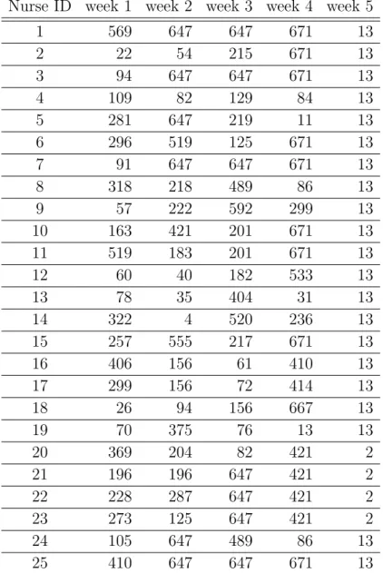
In the pattern-based formulation, the value k is set to 7; that is, a period corresponds to 1 week. Table 2 lists the number of feasible shift patterns for each nurse in 1 week. We can see that the number depends on the tightness of the type (b) nurse constraints concerning each nurse.
We also attempted to enumerate optimal solutions by using the “populate” option of CPLEX. However, only two optimal solutions were output in 10 hours with the basic for-mulation, and only one with the pattern-based formulation.
3. Generating Many Optimal Solutions
Let us consider a situation in which a scheduler has obtained an optimal solution ˆσ, and
assume that the scheduler wants to change the schedules of some nurses. In this situation, it would be helpful to know in advance which modifications are likely to cause violations of shift and/or nurse constraints. To obtain such information, we generate many optimal solutions around ˆσ and examine their features. In this section, we explain how to generate
many different optimal solutions.
For a given NSP instance, we define an optimal-solution space graph, which is an undi-rected graph with node setS consisting of all optimal solutions to the instance. Arcs connect two solution nodes σ and σ′ such that σi ̸= σi′ holds for some nurse i∈ I, and σi′ = σi′′ holds for all the other nurses i′ ∈ I \ {i}. In other words, the difference between σ and σ′ is only in the schedule for one nurse. Starting with a given optimal solution ˆσ, we can generate
different optimal solutions by traversing the optimal-solution space graph. Note that this approach is not guaranteed to generate every optimal solution, because an optimal-solution space graph is not necessarily connected.
In traversing the optimal-solution space graph, we must enumerate nodes that connect to the currently visited node. In our approach, for a given feasible solution σ of an NSP instance and a specific nurse i ∈ I, we consider the problem of optimizing the schedule of nurse i while keeping those of the other nurses the same. We denote this problem as NSP(σ, i) and call σ the seed solution (or the seed schedule). The following describes a method for enumerating optimal solutions to NSP(σ, i) [2].
This method is based on the pattern-based formulation. NSP(σ, i) can be formulated similarly to the original NSP, but it is different in that the decision variables λi′wp for nurses i′ other than i are fixed according to the seed schedule σi′. For each combination of g ∈ G, d ∈ D, and s ∈ S, let n′gds be the number of nurses i′ ∈ Ig \ {i} to whom s is assigned on d in σ. Then, assuming that nurse i has not yet been assigned any pattern (i.e.,
λiwp = 0 for all w ∈ W, p ∈ Piw), the tentative objective value f0 is given by f0 = ∑ g∈G ∑ d∈D ∑ s∈S max{0, α−gds(albgds− n′gds), α+gds(n′gds− aubgds)}.
Table 2: Numbers of feasible shift patterns for each week for each nurse Nurse ID week 1 week 2 week 3 week 4 week 5
1 569 647 647 671 13 2 22 54 215 671 13 3 94 647 647 671 13 4 109 82 129 84 13 5 281 647 219 11 13 6 296 519 125 671 13 7 91 647 647 671 13 8 318 218 489 86 13 9 57 222 592 299 13 10 163 421 201 671 13 11 519 183 201 671 13 12 60 40 182 533 13 13 78 35 404 31 13 14 322 4 520 236 13 15 257 555 217 671 13 16 406 156 61 410 13 17 299 156 72 414 13 18 26 94 156 667 13 19 70 375 76 13 13 20 369 204 82 421 2 21 196 196 647 421 2 22 228 287 647 421 2 23 273 125 647 421 2 24 105 647 489 86 13 25 410 647 647 671 13
The objective value with the shift patterns of i taken into consideration is calculated by ∑ w∈W ∑ p∈Piw fwpλiwp+ f0 by using fwp (w ∈ W, p ∈ Piw) defined as fwp= ∑ g∈µi ∑ d∈Dw ∑ s∈S ∆gdsδp,d−(w−1)k,s,
which represents the contribution of p selected as i’s shift pattern on period w to the objective function, where µi denotes the set of groups containing i and ∆gds is given by
∆gds = −α− gds if n′gds < a lb gds, α+gds if n′gds ≥ aubgds, 0 otherwise.
With the above notation, NSP(σ, i) is formulated as follows:
Minimize ∑ w∈W ∑ p∈Piw fwpλiwp+ f0 (3.1) subject to blbis ≤ ∑ w∈W ∑ p∈Piw ρpsλiwp ≤ bubis, s∈ S (3.2)
λi,w−1,p′ + λiwp≤ 1, w∈ W \ {1}, p ∈ Piw, p′ ∈ Pi,w−1∩ Rp (3.3) ∑
p∈Piw
λiwp = 1, w∈ W (3.4)
λiwp∈ {0, 1}, w∈ W, p ∈ Piw. (3.5)
To solve NSP(σ, i), we utilize a directed acyclic network that we call a shift-pattern network. Let Vw be defined as {(w, p) | p ∈ Piw}, and the node set V be given by the union of |W | sets Vw (w∈ W ) and the set of source and sink nodes. We denote a node in Vw also by (w, p). The arc set A is the union of the following three sets of arcs: (i) the set of arcs from the source to each node in V1, (ii) the set of arcs from each node (w− 1, p′) ∈ Vw−1 to each node (w, p) ∈ Vw such that p′ ∈ R/ p holds (w ∈ W \ {1}), and (iii) the set of arcs from each node in V|W | to the sink. Note that any path from the source to the sink on the network contains one node (w, pw) from each Vw. The sequence (p1, p2, . . . , p|W |) of the shift patterns represents a schedule for nurse i that satisfies nurse constraints of types (b) and (c). Conversely, any such schedule is represented by a path from the source to the sink.
For each arc (u, v) ∈ A, we define its length luv as follows: luv = 0 if v is the sink node; otherwise, luv = fwp, supposing v = (w, p). Then, the length of a path from the source to the sink plus f0 gives the objective value of the corresponding schedule. Because the schedule represented by a shortest path from the source to the sink may be infeasible due to avoiding constraints (3.2), to solve NSP(σ, i) we apply a k-shortest-path algorithm to the shift-pattern network while checking the feasibility of paths obtained during the computation.
As described below, in this paper, we consider NSP(σ, i) only for an optimal solution σ to the original NSP. In our experiments using Ikegami-3shift-DATA1, the shortest path length plus f0 always coincided with the objective value of σ. This means that we can enumerate
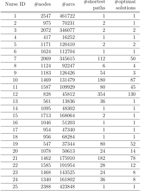
Table 3: Numbers of nodes, arcs, shortest paths, and optimal solutions in the shift-pattern network for each nurse
Nurse ID #nodes #arcs #shortest paths #optimal solutions 1 2547 461722 1 1 2 975 70231 2 1 3 2072 346077 2 2 4 417 16252 1 1 5 1171 120410 2 2 6 1624 112704 1 1 7 2069 345615 112 50 8 1124 92247 6 4 9 1183 126426 54 3 10 1469 131479 180 87 11 1587 109929 80 45 12 828 45812 354 130 13 561 13836 36 1 14 1095 48302 1 1 15 1713 168064 2 1 16 1046 51203 1 1 17 954 47340 1 1 18 956 68284 1 1 19 547 37344 80 52 20 1078 50613 24 14 21 1462 175910 182 78 22 1585 191954 28 12 23 1468 143525 24 8 24 1340 161802 36 8 25 2388 423848 1 1
all the optimal solutions to NSP(σ, i) by traversing arcs contained in some shortest path backward from the sink while checking the feasibility for every shortest path.
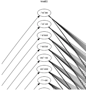
For Ikegami-3shift-DATA1, we constructed shift-pattern networks to solve NSP(σ(1), i) for each nurse i, where the seed solution σ(1) is an optimal solution obtained by CPLEX. The computational time required to generate the shift-pattern networks is about 12 seconds in total. The second and third columns in Table 3 list the numbers of nodes and arcs in the shift-pattern network for each NSP(σ(1), i). As an example, Figure 2 shows the network for nurse 4, which has the fewest nodes among those for all nurses. Figure 3 is an enlarged view of part of the network.
Table 3 also gives the number of shortest paths in the shift-pattern network and the number of optimal solutions. Because the original schedule σi for nurse i is an optimal solution to NSP(σ, i) such that NSP(σ, i) has more than one optimal schedule, we can obtain another optimal schedule σ′ from σ by replacing σi with another optimal solution to NSP(σ, i). Because the total number of optimal solutions in the last column of Table 3 is 506, we can obtain 481 optimal solutions in total from σ(1), where 481 (= 506− 25) is derived from the total number of optimal solutions by excluding the seed solution σ(1) for each nurse. This means that 481 nodes are adjacent to σ(1) in the optimal-solution space graph.
We can see that the numbers of shortest paths and optimal solutions depend on the tightness of the shift constraints, rather than the numbers of nodes and arcs. For example, for nurses i = 1, . . . , 6, 14, . . . , 18, and 25, NSP(σ(1), i) has fewer shortest paths than the others, which results in fewer optimal solutions. This is mainly because they are more tightly restricted by shift constraints; they are categorized as leaders, and there exist some groups
g ∈ G consisting of some of them. We conducted the same experiment using seven other
optimal solutions σ(2), . . . , σ(8) as seed solutions. The results are given in Table 4. The same tendency is always observed, which indicates that the schedules for the leaders are difficult to modify while maintaining optimality. For other nurses, the number of optimal solutions is highly dependent on the seed solution.
Next, to see how many optimal solutions are generated by our approach, we conducted a computational experiment for Ikegami-3shift-DATA1. Our approach generated more than 70 million optimal solutions by checking a very small part of the optimal-solution space graph. Although it is difficult to estimate the number of optimal solutions, it turns out that this instance has very many. However, we found that these solutions have many common patterns; for 66 out of the 25× 5 = 125 pairs of nurse i ∈ I and period w ∈ W , the same pattern is used in all the generated solutions.
4. Extracting Useful Information from Different Optimal Solutions
To analyze the features of optimal solutions generated by our approach, we applied a breadth-first search to the optimal-solution space graph, using each of the eight optimal solutions in Table 4 as the starting solution ˆσ. In this experiment, we suppose that only
the schedules for nurses 14–25 can be modified, and for the other nurses 1–13, any optimal solution to be generated has the same schedule as ˆσ. The numbers of generated optimal
solutions are given in Table 5, where Sl denotes the set of generated optimal solutions σ such that the distance from ˆσ in the optimal-solution space graph is less than or equal to l (note that S0 consists of ˆσ only). Note that the number of optimal solutions depends on the starting solution, but for all cases, there exist many optimal solutions whose distance from the starting solution is even at most four.
Table 4: Numbers of optimal solutions to NSP(σ, i) for different seed solutions σ seed solution σ Nurse ID σ(1) σ(2) σ(3) σ(4) σ(5) σ(6) σ(7) σ(8) 1 1 1 3 1 2 1 3 1 2 1 1 1 1 1 1 2 1 3 2 1 1 3 1 1 1 2 4 1 1 1 1 2 1 2 1 5 2 1 1 1 2 1 1 1 6 1 1 1 1 2 2 1 1 7 50 5 28 9 32 16 6 20 8 4 37 7 286 4 151 151 10 9 3 47 9 3 29 6 7 66 10 87 20 4 7 57 16 193 86 11 45 7 78 184 16 19 15 24 12 130 200 20 10 23 189 54 172 13 1 1 8 1 11 3 1 18 14 1 1 1 1 2 1 1 1 15 1 1 1 1 1 1 1 2 16 1 1 1 1 1 1 1 1 17 1 1 1 1 1 1 1 1 18 1 1 1 1 1 2 1 1 19 52 1 2 10 5 113 119 26 20 14 11 12 2 30 18 5 4 21 78 8 6 9 15 5 12 20 22 12 61 45 40 111 11 82 8 23 8 53 21 5 5 17 6 66 24 8 10 2 20 9 41 8 26 25 1 1 3 3 1 3 2 3
Table 5: Numbers of generated optimal solutions for different starting solutions starting solution ˆσ σ(1) σ(2) σ(3) σ(4) σ(5) σ(6) σ(7) σ(8) |S0| 1 1 1 1 1 1 1 1 |S1| 167 139 85 83 170 203 228 148 |S2| 15,135 6,931 3,145 3,937 8077 17,824 24,509 9,810 |S3| 790,043 158,867 76,781 114,087 182,458 891,387 1,263,067 365,401 |S4| 24,671,253 2,187,241 1,062,604 1,694,237 2,175,638 27,277,865 25,466,799 8,267,515
Figure 2: Example of a shift-pattern network
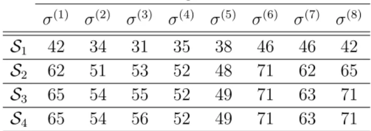
To see the variety of shift assignments among the solutions, for each nurse and each day, we summarized the numbers of solutions in which each type of shift appears. As an example, for the case of ˆσ = σ(2), we give the results for S
4 in Table 6. We observed that the individual schedules for nurses 14–18 and 25 (who are leaders) are common in all the optimal solutions in S4, whereas possible shifts are quite limited for each day for the other nurses; there are only one or two possible shifts, and in the latter case, they are “day-off” (/) or “day shift” (–). This information would be helpful for the scheduler, allowing him or her to see which assignment in the schedule would be easier to change while maintaining optimality.
It is generally time-consuming to generate a large number of solutions. In the above example, the computational time for generating solutions depends on the starting node ˆσ.
In the case of ˆσ = σ(6)(for which the most solutions were generated among the eight), all the solutions inS2were generated in less than 20 seconds, whereas more than 1 hour was required forS3 and it took almost 1 month forS4. However, if we focus on diversity in shifts assigned to each nurse on each day, the differences amongS2,S3, andS4are not large. To demonstrate this, Table 7 shows the number of pairs of (i, d) (i∈ {14, . . . , 25}, d ∈ {1, . . . , 30}) such that more than one shift appears in some optimal solution inS1, . . . ,S4 (i.e., the shift is not fixed to the original one, but there exists an alternative shift). This observation indicates that just by generating solutions in S2, it became possible to guess to some extent which part of the schedule could be modified. It is also promising to randomly truncate some nodes in the breadth-first search instead of completely traversing all nodes around the starting node. Even optimal solutions generated in this manner are expected to give a good approximation.
T able 6: Num b ers of app earances of eac h shift (S 4 ) n urse shift 1 2 3 4 5 6 7 8 9 10 11 12 13 14 15 16 17 18 19 20 21 22 23 24 25 26 27 28 29 30 / 0 0 0 2,187,241 0 0 0 2,187,241 0 0 2,187,241 2,187,241 2,187,241 0 0 0 0 2,187,241 2,187,241 0 0 0 0 0 0 2,187,241 2,187,241 0 0 0 – 0 0 0 0 2,187,241 0 0 0 2,187,241 0 0 0 0 2,187,241 2,187,241 0 0 0 0 2,187,241 2,187,241 2,187,241 2,187,241 0 0 0 0 2,187,241 2,187,241 0 14 e 2,187,241 2,187,241 2,187,241 0 0 2,187,241 2,187,241 0 0 0 0 0 0 0 0 0 0 0 0 0 0 0 0 0 0 0 0 0 0 2,187,241 n 0 0 0 0 0 0 0 0 0 0 0 0 0 0 0 2,187,241 2,187,241 0 0 0 0 0 0 2,187,241 2,187,241 0 0 0 0 0 + 0 0 0 0 0 0 0 0 0 2,187,241 0 0 0 0 0 0 0 0 0 0 0 0 0 0 0 0 0 0 0 0 / 0 0 2,187,241 0 0 2,187,241 0 0 0 0 2,187,241 0 0 2,187,241 0 0 2,187,241 2,187,241 0 0 0 2,187,241 0 0 2,187,241 0 0 0 0 2,187,241 – 2,187,241 2,187,241 0 2,187,241 0 0 2,187,241 2,187,241 0 0 0 0 0 0 2,187,241 2,187,241 0 0 0 0 0 0 2,187,241 2,187,241 0 2,187,241 2,187,241 0 0 0 15 e 0 0 0 0 2,187,241 0 0 0 0 0 0 2,187,241 2,187,241 0 0 0 0 0 2,187,241 2,187,241 2,187,241 0 0 0 0 0 0 0 0 0 n 0 0 0 0 0 0 0 0 2,187,241 2,187,241 0 0 0 0 0 0 0 0 0 0 0 0 0 0 0 0 0 2,187,241 2,187,241 0 + 0 0 0 0 0 0 0 0 0 0 0 0 0 0 0 0 0 0 0 0 0 0 0 0 0 0 0 0 0 0 / 0 0 2,187,241 2,187,241 0 0 2,187,241 0 0 0 2,187,241 0 0 0 0 2,187,241 2,187,241 0 0 2,187,241 0 0 0 2,187,241 0 0 2,187,241 0 0 0 – 0 0 0 0 2,187,241 2,187,241 0 0 0 0 0 2,187,241 0 0 0 0 0 2,187,241 2,187,241 0 0 0 0 0 2,187,241 0 0 2,187,241 2,187,241 2,187,241 16 e 0 0 0 0 0 0 0 2,187,241 2,187,241 2,187,241 0 0 0 0 0 0 0 0 0 0 0 2,187,241 2,187,241 0 0 2,187,241 0 0 0 0 n 2,187,241 2,187,241 0 0 0 0 0 0 0 0 0 0 0 2,187,241 2,187,241 0 0 0 0 0 0 0 0 0 0 0 0 0 0 0 + 0 0 0 0 0 0 0 0 0 0 0 0 2,187,241 0 0 0 0 0 0 0 2,187,241 0 0 0 0 0 0 0 0 0 / 2,187,241 0 0 0 0 0 2,187,241 2,187,241 2,187,241 0 0 2,187,241 0 0 0 2,187,241 0 0 0 2,187,241 2,187,241 0 0 0 0 0 0 2,187,241 2,187,241 0 – 0 2,187,241 2,187,241 0 0 0 0 0 0 2,187,241 0 0 0 0 0 0 2,187,241 0 0 0 0 2,187,241 2,187,241 0 0 0 0 0 0 2,187,241 17 e 0 0 0 2,187,241 0 0 0 0 0 0 2,187,241 0 0 2,187,241 2,187,241 0 0 0 0 0 0 0 0 2,187,241 2,187,241 0 0 0 0 0 n 0 0 0 0 2,187,241 2,187,241 0 0 0 0 0 0 0 0 0 0 0 2,187,241 2,187,241 0 0 0 0 0 0 2,187,241 2,187,241 0 0 0 + 0 0 0 0 0 0 0 0 0 0 0 0 2,187,241 0 0 0 0 0 0 0 0 0 0 0 0 0 0 0 0 0 / 2,187,241 2,187,241 0 0 2,187,241 0 0 0 2,187,241 2,187,241 2,187,241 0 0 0 2,187,241 0 0 0 2,187,241 0 0 0 0 2,187,241 2,187,241 0 0 0 0 0 – 0 0 2,187,241 2,187,241 0 2,187,241 0 0 0 0 0 2,187,241 2,187,241 2,187,241 0 0 0 0 0 0 2,187,241 0 0 0 0 2,187,241 0 0 0 0 18 e 0 0 0 0 0 0 0 0 0 0 0 0 0 0 0 2,187,241 2,187,241 2,187,241 0 0 0 0 0 0 0 0 2,187,241 2,187,241 2,187,241 0 n 0 0 0 0 0 0 2,187,241 2,187,241 0 0 0 0 0 0 0 0 0 0 0 0 0 2,187,241 2,187,241 0 0 0 0 0 0 2,187,241 + 0 0 0 0 0 0 0 0 0 0 0 0 0 0 0 0 0 0 0 2,187,241 0 0 0 0 0 0 0 0 0 0 / 0 2,108,229 0 79,012 22,299 2,004,413 0 0 2,187,241 109,880 0 0 2,187,241 161,011 0 0 2,187,241 0 0 0 0 0 2,187,241 2,187,241 2,187,241 2,187,241 0 0 1,929,891 0 – 2,187,241 79,012 2,187,241 2,108,229 2,164,942 182,828 0 0 0 2,077,361 2,187,241 0 0 2,026,230 2,187,241 0 0 2,187,241 2,187,241 2,187,241 0 0 0 0 0 0 2,187,241 2,187,241 257,350 2,187,241 19 e 0 0 0 0 0 0 0 2,187,241 0 0 0 2,187,241 0 0 0 0 0 0 0 0 0 0 0 0 0 0 0 0 0 0 n 0 0 0 0 0 0 0 0 0 0 0 0 0 0 0 0 0 0 0 0 2,187,241 2,187,241 0 0 0 0 0 0 0 0 + 0 0 0 0 0 0 2,187,241 0 0 0 0 0 0 0 0 2,187,241 0 0 0 0 0 0 0 0 0 0 0 0 0 0 / 0 0 0 0 2,187,241 0 0 2,187,241 2,187,241 731,362 96,283 153,835 237,119 1,429,648 0 0 2,187,241 2,187,241 2,187,241 6,055 0 1,206,866 0 980,375 0 299,543 1,293,778 1,274,069 501,163 0 – 2,187,241 0 0 0 0 2,187,241 0 0 0 1,455,879 2,090,958 2,033,406 1,950,122 757,593 0 0 0 0 0 2,181,186 2,187,241 980,375 2,187,241 1,206,866 2,187,241 1,887,698 893,463 913,172 1,686,078 0 20 e 0 2,187,241 2,187,241 2,187,241 0 0 2,187,241 0 0 0 0 0 0 0 0 0 0 0 0 0 0 0 0 0 0 0 0 0 0 0 n 0 0 0 0 0 0 0 0 0 0 0 0 0 0 2,187,241 2,187,241 0 0 0 0 0 0 0 0 0 0 0 0 0 0 + 0 0 0 0 0 0 0 0 0 0 0 0 0 0 0 0 0 0 0 0 0 0 0 0 0 0 0 0 0 2,187,241 / 0 0 2,187,241 2,187,241 223,093 0 969,776 2,187,241 0 0 2,187,241 803,879 0 0 2,187,241 530,830 0 0 0 0 2,187,241 0 0 2,187,241 0 0 644,092 1,311,231 1,273,968 0 – 0 0 0 0 1,964,148 2,187,241 1,217,465 0 2,187,241 0 0 1,383,362 0 0 0 1,656,411 2,187,241 2,187,241 0 0 0 0 0 0 2,187,241 2,187,241 1,543,149 876,010 913,273 0 21 e 0 0 0 0 0 0 0 0 0 2,187,241 0 0 2,187,241 2,187,241 0 0 0 0 0 0 0 2,187,241 2,187,241 0 0 0 0 0 0 0 n 2,187,241 2,187,241 0 0 0 0 0 0 0 0 0 0 0 0 0 0 0 0 2,187,241 2,187,241 0 0 0 0 0 0 0 0 0 0 + 0 0 0 0 0 0 0 0 0 0 0 0 0 0 0 0 0 0 0 0 0 0 0 0 0 0 0 0 0 2,187,241 / 0 4,765 0 1,297,295 1,386,080 576,872 0 392,471 2,187,241 0 0 2,187,241 2,187,241 895,323 0 0 0 2,187,241 0 0 0 2,187,241 0 0 2,187,241 800,750 329,290 1,010,766 1,174,447 0 – 0 2,182,476 2,187,241 889,946 801,161 1,610,369 2,187,241 1,794,770 0 0 0 0 0 1,291,918 2,187,241 2,187,241 0 0 0 0 0 0 2,187,241 0 0 1,386,491 1,857,951 1,176,475 1,012,794 0 22 e 0 0 0 0 0 0 0 0 0 0 0 0 0 0 0 0 2,187,241 0 2,187,241 2,187,241 2,187,241 0 0 2,187,241 0 0 0 0 0 0 n 0 0 0 0 0 0 0 0 0 2,187,241 2,187,241 0 0 0 0 0 0 0 0 0 0 0 0 0 0 0 0 0 0 0 + 2,187,241 0 0 0 0 0 0 0 0 0 0 0 0 0 0 0 0 0 0 0 0 0 0 0 0 0 0 0 0 2,187,241 / 697,982 0 0 0 2,187,241 2,187,241 0 0 2,187,241 2,187,241 545,672 43,488 614,730 1,056,623 890,059 360,573 0 0 2,187,241 1,255,290 1,003,054 553,193 0 737,033 0 0 0 2,187,241 407,046 0 – 1,489,259 2,187,241 0 0 0 0 2,187,241 2,187,241 0 0 1,641,569 2,143,753 1,572,511 1,130,618 1,297,182 1,826,668 2,187,241 0 0 931,951 1,184,187 1,634,048 2,187,241 1,450,208 0 0 0 0 1,780,195 0 23 e 0 0 0 0 0 0 0 0 0 0 0 0 0 0 0 0 0 2,187,241 0 0 0 0 0 0 2,187,241 2,187,241 2,187,241 0 0 0 n 0 0 2,187,241 2,187,241 0 0 0 0 0 0 0 0 0 0 0 0 0 0 0 0 0 0 0 0 0 0 0 0 0 0 + 0 0 0 0 0 0 0 0 0 0 0 0 0 0 0 0 0 0 0 0 0 0 0 0 0 0 0 0 0 2,187,241 / 0 2,187,241 2,187,241 0 0 0 2,187,241 236,659 0 0 0 2,187,241 178,558 0 0 0 0 0 2,187,241 2,187,241 0 0 0 88,447 2,187,241 2,187,241 1,750,259 1,564,694 273,852 0 – 0 0 0 2,187,241 0 0 0 1,950,582 2,187,241 2,187,241 0 0 2,008,683 2,187,241 0 0 0 0 0 0 2,187,241 2,187,241 2,187,241 2,098,794 0 0 436,982 622,547 1,913,389 2,187,241 24 e 2,187,241 0 0 0 2,187,241 2,187,241 0 0 0 0 2,187,241 0 0 0 2,187,241 2,187,241 0 0 0 0 0 0 0 0 0 0 0 0 0 0 n 0 0 0 0 0 0 0 0 0 0 0 0 0 0 0 0 2,187,241 2,187,241 0 0 0 0 0 0 0 0 0 0 0 0 + 0 0 0 0 0 0 0 0 0 0 0 0 0 0 0 0 0 0 0 0 0 0 0 0 0 0 0 0 0 0 / 0 2,187,241 0 0 2,187,241 2,187,241 0 0 0 2,187,241 0 0 0 2,187,241 2,187,241 0 0 0 0 0 0 2,187,241 2,187,241 0 0 2,187,241 0 0 0 0 – 2,187,241 0 0 0 0 0 2,187,241 2,187,241 0 0 2,187,241 0 0 0 0 2,187,241 2,187,241 2,187,241 2,187,241 0 0 0 0 2,187,241 2,187,241 0 2,187,241 0 0 0 25 e 0 0 0 0 0 0 0 0 2,187,241 0 0 0 0 0 0 0 0 0 0 0 0 0 0 0 0 0 0 2,187,241 2,187,241 2,187,241 n 0 0 2,187,241 2,187,241 0 0 0 0 0 0 0 2,187,241 2,187,241 0 0 0 0 0 0 2,187,241 2,187,241 0 0 0 0 0 0 0 0 0 + 0 0 0 0 0 0 0 0 0 0 0 0 0 0 0 0 0 0 0 0 0 0 0 0 0 0 0 0 0 0
Table 7: Numbers of nurse–day pairs for which an alternative shift exists Starting solution ˆσ σ(1) σ(2) σ(3) σ(4) σ(5) σ(6) σ(7) σ(8) S1 42 34 31 35 38 46 46 42 S2 62 51 53 52 48 71 62 65 S3 65 54 55 52 49 71 63 71 S4 65 54 56 52 49 71 63 71
To confirm performance, we applied our generation method to three other real-world instances: Ikegami-3shift-DATA1.1, Ikegami-3shift-DATA1.2, and Ikegami-2shift-DATA2 [12]. In this experiment, we assume that schedules for all nurses can be modified. The computational results show that all generated schedules for S1 and S2 were completed in less than 1 second and 6 hours, respectively. We also observe that many solutions exist in
S2 for all tested instances. See Appendix A for more details on the computational results. 5. Conclusions
In this paper, we considered an improved approach to the nurse scheduling problem (NSP), aiming at optimization techniques that should prove more useful. To solve the NSP un-der real-world situations in Japan, we consiun-dered ideas providing useful information for modifications possibly needed in the future.
Aiming at obtaining information that would be useful for decision-makers when manually modifying an obtained optimal schedule, we proposed a method for generating many optimal schedules. In our computational experiments with a benchmark instance, we observed that there exist many different optimal schedules around a given one. However, their differences involve somewhat limited numbers of nurses and days. Moreover, for some nurses, shift patterns are common among all generated optimal solutions. We expect these features of optimal solutions to provide decision-makers with clues regarding which parts of a schedule can be modified.
In our experiments with Ikegami-3shift-DATA1, a huge number of optimal solutions were generated by the method described in this paper. However, this is not always the case. When only a few optimal solutions exist, it would be better to modify the definition of the node set of an optimal-solution space graph so that it includes near-optimal solutions in addition to optimal ones. Another definition of the arc set is also possible. For example, two optimal (or near-optimal) solutions are connected if they have common individual schedules for all nurses except two. Although this necessitates improvements to the method described in Section 3, more useful information might be obtained.
In conclusion, we proposed a method for generating large numbers of optimal solutions based on a given optimal solution. We also demonstrated the utility of method, show-ing that useful information for decision-makers can be extracted by slightly modifyshow-ing an obtained optimal schedule, specifically by setting the maximum distance from a seed solu-tion. Our method thus provides information within short computational times. However, decision-makers may also at first require several optimal solutions with different features for selection of the most desired one. One important future research direction is to consider methods for generating many optimal or near-optimal solutions with features different from one another by considering the definition of difference or distance among solutions.
References
[1] A.A. El Adoly, M. Gheith, and M.N. Fors: A new formulation and solution for the nurse scheduling problem: A case study in Egypt. Alexandria Engineering Journal, 57 (2018), 2289–2298.
[2] H. Akita and A. Ikegami: A network representation of feasible solution space for a subproblem of nurse scheduling. Proceedings of the Institute of Statistical Mathematics, 61 (2013), 79–95.
[3] P. Brucker, E.K. Burke, T. Curtois, R. Qu, and G.V. Berghe: A shift sequence based approach for nurse scheduling and a new benchmark dataset. Journal of Heuristics, 16 (2010), 559–573.
[4] G. Baskaran, A. Bargiela, and R. Qu: Using branch and bound to solve the nurse scheduling problem. Proceedings of 2014 International Conference on Artificial
Intelli-gence & Manufacturing Engineering, IIE ICAIME2014, 2014, 203–209.
[5] E.K. Burke, P. De Causmaecker, G.V. Berghe, and H. Van Landeghem: The state of the art of nurse rostering. Journal of Scheduling, 7 (2004), 441–499.
[6] M. Bagheri, A.G. Devin, and A. Izanloo: An application of stochastic programming method for nurse scheduling problem in real word hospital. Computers & Industrial
Engineering, 96 (2016), 192–200.
[7] P. Brucker, R. QU, and E.K. Burke: Personnel scheduling: Models and complexity.
European Journal of Operational Research, 210 (2011), 467–473.
[8] T. Curtois: Employee shift scheduling benchmark data sets.
http://www.schedulingbenchmarks.org/nrp/ (accessed 2020-11-16).
[9] B. Cheang, H. Li, A. Lim, and B. Rodrigues: Nurse rostering problems—A biblio-graphic survey. European Journal of Operational Research, 151 (2003), 447–460. [10] M. Hamid, F. Barzinpour, M. Hamid, and S. Mirzamohammadi: A multi-objective
mathematical model for nurse scheduling problem with hybrid DEA and augmented
ϵ-constraint method: A case study. Journal of Industrial and Systems Engineering, 11
(2018), 98–108.
[11] A. Ikegami, M. Aizawa, M. Ohkura, B. Wakasa, N. Matsudaira, and R. Kosugoh: A preliminary study on the development of a scheduling system for hospital nurses.
Journal of Science of Labour, 71 (1995), 413–423. (in Japanese)
[12] A. Ikegami and A. Niwa: A subproblem-centric model and approach to the nurse scheduling problem. Mathematical Programming, 97 (2003), 517–541.
[13] A. Ikegami and A. Niwa: A hyper-heuristic using grasp with path-relinking: A case study of the nurse rostering problem. Interdisciplinary Advances in Information
Tech-nology Research, 89 (2013), 89–99.
[14] A. Ikegami, A. Niwa, and M. Ohkura: Nurse scheduling problem in Japan.
Communi-cations of the Operations Research Society of Japan, 41 (1996), 436–442. (in Japanese)
[15] H. Jafari, S. Bateni, P. Daneshvar, S. Bateni, and H. Mahdioun: Fuzzy mathemati-cal modeling approach for the nurse scheduling problem: A case study. International
Journal of Fuzzy Systems, 18 (2016), 320–332.
[16] JP. M´etivier, P. Boizumault, and S. Loudni: Solving nurse rostering problems using soft global constraints. International Conference on Principles and Practice of Constraint
Programming, 2009, 73–87.
network programming. European Journal of Operational Research, 104 (1998), 582– 592.
[18] J. Van den Bergh, J. Beli¨en, P. De Bruecker, E. Demeulemeester, and L. De Boeck: Personnel scheduling: A literature review. European Journal of Operational Research, 226 (2013), 367–385.
[19] S. Zanda, P. Zuddas, and C. Seatzu: Long term nurse scheduling via a decision support system based on linear integer programming: A case study at the University Hospital in Cagliari. Computers & Industrial Engineering, 126 (2018), 337–347.
A. Generating Optimal Solutions for Different Instances
Assuming that all nurse schedules can be modified, we also tested the generation approach on four real-world instances: DATA1, DATA1.1, Ikegami-3shift-DATA1.2 and Ikegami-2shift-DATA2, which are regarded as typical instances in Japan. In-stances 3shift-DATA1.1 and 3shift-DATA1.2 are generated from Ikegami-3shift-DATA1 by introducing more on-site requirements to type-(b) nurse constraints in or-der to consior-der additional preferences. Thus, sets F0 and F1 contain more elements than in Ikegami-3shift-DATA1. Instance Ikegami-2shift-DATA deals with two-shift system schedul-ing for 30 days and 28 nurses. All instances are available online at [8].
In this experiment, we chose arbitrarily one seed solution for each instance (for Ikegami-3shift-DATA1, σ(7)).
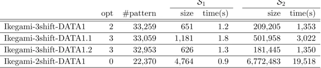
Table 8 shows the results of generating optimal solutions inS1 andS2. For each instance, we provide optimal solution values (“opt”) and the total number of feasible shift patterns (“#pattern”) for each week for each nurse. For S1 and S2, we provide the number of optimal solutions (“size”) and the CPU runtime in seconds (“time”) required to generate all corresponding solutions.
Table 8: Results of generating optimal solutions for different instances
S1 S2
opt #pattern size time(s) size time(s)
Ikegami-3shift-DATA1 2 33,259 651 1.2 209,205 1,353 Ikegami-3shift-DATA1.1 3 33,059 1,181 1.8 501,958 3,022 Ikegami-3shift-DATA1.2 3 32,953 626 1.3 181,445 1,350 Ikegami-2shift-DATA1 0 22,370 4,764 0.9 6,772,483 19,518 Atsuko Ikegami Seikei University 3-3-1 Kichijoji-Kitamachi, Musashino-shi Tokyo 180-8633, Japan E-mail: [email protected]