立命館学術成果リポジトリ

(1)

Introducing

Philip Sallis

• Undergraduate degrees in NZ. PhD in London, England

• Academic positions in UK, Australia, NZ

• Visiting and Adjunct Professorships in UK, HK, USA and Chile

• Research in geophysics and geo spatial systems, software

engineering, computational linguistics

• Joined AUT in 1999 as DVC (Pro Chancellor)

• From today

– Director Geoinformatics Research Centre

(2)

AUT

Auckland University of Technology

140 years old but established as a university in Jan 2000

26,000 students (4000 international students)

15% postgraduate (Masters, PhDs, some PG Diploma)

4 Faculties on three campuses:

Business and Law

Design and Creative Technologies

Health and Environmental Sciences

Humanities

12 Research Institutes and 10 Research Centres

Technology Park

Business Innovation and Enterprise

Research Commercialisation

(3)

The

Geoinformatics Research Centre

www.geomaticsresearch.org

School of Computing and Mathematical Sciences

Auckland University of Technology

New Zealand

www.aut.ac.nz

Professor Philip Sallis

(4)

GRC Profile

established August 2007

13 AUT 3 full-time

+ 3 associates

+ 1 administrator

+ 2 interns

8 more scientists

in 5 countries

6 vineyards

in 4 countries

2+5 PhD

students

Publications

Electrical tools and

lab equipment

Server, computers,

printers, cameras

sensors, analysers

(5)

Expertise

• Mathematics and Statistics

• Computer Science & Software Engineering

• Electrical Engineering

• Biology and Zoology

• Forestry and Environmental Science

• Geodetic Science and Geocomputation

• Oenology (enology)...wine science

• Viticulture

• Climatology

(6)

Current GRC projects

staff and students

• Data mining – wine quality influence factors

–

climate and atmospheric data processing with neural networks

–

data relationship depiction and result visualisation methods

• Text and Audio Mining

–

taxonomy construction from wine characteristic descriptions (text)

–

coincidence of verbal tasting keyword descriptions of wine with expert database of terms (audio)

–

analysis of discourse relating to wine quality (comparative study in Spanish and English)

• Geocomputation

–

spatial DB construction

–

Remote sensing, image rendering and processing

–

Image processing method with spectrum analysis of fruit colour and taste

–

sensor construction, data logging, signal processing and wireless communications technologies

–

prototype construction of robotic multi-sensor device

–

real-time data ingestion infrastructure design and operation

• Geometrics

–

equations and algorithms for geo-spatial measurement & modelling

• Geographic Information Systems applications

–

forestry management

–

health service delivery

–

tourism provision

(7)

The Main Project

‘Eno-Humanas’

Precision Agronomy

Data Acquisition

Modelling and Prediction

Precise data Imprecise data

(8)

The Main Project

Spawns sub-projects

Image Processing Data Mining Audio Mining Frost Prediction Irrigation Management Remote Sensing Climate Trends GIS Applications Sensor Technologies

(9)

An International Research Collaboration

integrates precision data from sensors, with telemetry

and software technologies plus human sensory

perception (opinion) data

Uruguay

Chile

Japan

USA

New Zealand

‘Eno-Humanas’

Environmental factors influencing good grape growth

for the production of great wine…an empirical study

(10)

Eno-Humanas

It all began in 2007 with a question:

(11)

Four main variables for good grape

growth to make great wine

• Soil

• Climate

• Variety

• Terrain

(12)

The Matrix

(database)

Unique Key (concatenated )= time+date+long:lat

Vector data

Temperature

o

_C

Wind Speed

km/hr

Wind Direction

Ddd

Wind Chill

o

_C

Humidity

%

Dewpoint

o

_C

Solar Radiation

(Pyrheliometer for Photsynthetic Light Measurement)

umol/m

2

_/sec

Pollution factors (CO

₂

)

%

Rainfall

mm

Barometric Pressure

hpa

Soil Moisture

%

Soil Temperature

o

_C

Leaf Wetness

%

Sap Flow

(volume and speed)

Ltrs/min

Plant growth Rate

(Dendrometer)

%

(13)

Grape and wine characteristics relating to location, growing

conditions, climate and environment

(14)

Research Partners

• Universities

– Auckland University of Technology, New Zealand

– Universidad Catolica del Maule, Chile

– Universidad de Talca, Chile

– ZonAmercia, Montevideo, Uruguay

– University of California at Santa Barbara (UCSB)

– Asia Pacific University, Beppu, Japan

• Industry Partners

– EDA Systems, Irvine, California, USA

– Mahurangi River Winery, Auckland, New Zealand

– Kumeu River Winery, Henderson, New Zealand

– Casa Donoso Winery, Maule, Chile

– Santa Elisa Research Vineyard, Parral, Chile

– La Agricola Jackson Winery, Montevideo, Uruguay

– Fallbrook Winery, Irvine, Sth California

(15)

AUT: 36o_{51’ S 174}o_{52’ E} _{UCM: 33}o_{20’ N 131}o_{28’ E} _{Montevideo: 34}o_{53’ S 56}o_{04’ W}

(16)

© Mahurangi Winery Limited

Producers of fine New Zealand wines

(17)

(18)

Santa Elisa Experimental Organic Vineyard,

Parral, Valle de Maule

(19)

La Agricola Jackson, Montevideo, Uruguay

La Agrícola Jackson

(20)

Fallbrook Winery,

(21)

(22)

Technology Partners

• Colleagues in Electrical and Computer Engineering (AUT

and UCM)

• Commercial entities from whom we have purchased

equipment (La Crosse, Davis, Garmin, etc)

• A sensor technology design and development company

in Sth California (

Cog

net

ive Systems

)

(23)

Electronic Design Associates (EDA) Inc

(

Cog

net

ive

)

Irvine, California

www.cognetive.com

(24)

R

S

= Wireless Sensor (e.g. T, RH, Switch Closure)

R

= Mesh Repeater

G

= Internet Gateway

Cognetive

Wireless Sensor Topology

S

G

Internet

S

R

Output = RF and/or Serial

G

Output = Serial or Ethernet

S

Output = RF

(25)

The Eno-Humanas system

concept

(26)

…

Chile

USA

Japan

Uruguay

Data gathered by

sensors & uploaded to

GRC server in real time

Frost, irrigation,

harvest, crop

quality

Trend analysis, prediction

models, scenarios for crop

management

(27)

CLIMATE

A major factor is the

weather

Weather patterns are changing.

We can’t rely on historical data or

intuition as in previous times, so

prediction systems need to be

built using historical and current

real time data and micro climate

sensitivity.

(28)

Comparison of data from two locations only 5 kms apart

(29)

(30)

Casa Donoso & UCM atmospheric

pressure comparisons

(31)

Temperature Tracking for frost prediction

Temperature

-5,0 0,0 5,0 10,0 15,0 20,0 25,0 1 7 13 19 25 31 37 43 49 55 61 67 73 79 85 91 97 103 109 115

Temp. °C each hour

T e m p . °C

Frost 1 Frost 2 Frost 3

(32)

1.3°C

Global warming

changes ?

Are we having

frost tomorrow? When?

Questions and

Prediction

(33)

Using CNN for climate prediction

CLASSIFICATION NEURAL NETWORK … …

Prototype under construction

Identification of variables, collection, classification and

processing of data

(34)

Temperature and Humidity plots for frost prediction

and

SOM depictions of data dependencies for

(a) temperature, relative humidity, dew point, wind velocity and direction

(b) date, temperature, relative humidity, dew point, wind direction

0 10 20 30 40 50 60 70 80 90 100 1 4 7 10 13 16 19 22 25 28 31 34 37 40 43 46 49 Temperature Humidity 0 10 20 30 40 50 60 70 80 90 100 1 4 7 10 13 16 19 22 25 28 31 34 37 40 43 46 49 Temperature Humidity (a) (b)

(35)

Mineset Visualisations

(36)

Text and Data Mining

• To explore relationships between some

qualitative

data

and some

quantitative

data in a precision agronomy

research domain. That is, to explore explicit and implicit

data relationships between

human opinion

and

scientific

instrument data

(plant, soil and climate sensors).

• More specifically, to determine the strength of dependency

between comments made about

grape varieties

and their

growing conditions

, which includes their

geo-spatial

location

, in the pursuit of determining quality

(37)

Location and Condition

of the plants

Quality of the fruit

Opinion of the wine

Expert description of plants,

wine, growing conditions

Precise

Imprecise

Climate

Written

comments

Correlations

?

Wine characteristics

historically and now –

referenced by location

SOM

methods

(38)

Clusters from SOM analysis

SOM

100 nodes

Variety

quality

Growing

conditions

Geo-spatial,

climate, terrain,

soil data

Written comments

Dependency

values

k-1

F=∑ (tf x idf)

v=1 n

Word freq weight

Clusters of

correlated

data

Extraction

PCA

K-mean

wfw

Vector

Space

Model

(39)

Vector space model

(40)

0 2 4 6 8 10 12 14 16 C e n tr a l O ta g o H a w k e 's B a y K u m e u M a rl b o ro u g h M a rt in b o ro u g h M o u te re N e w Z e a la n d W a ip a ra W a ir a ra p a A w a te re C e n tr a l O ta g o H a w k e 's B a y M a rl b o ro u g h C e n tr a l O ta g o H a w k e 's B a y M a rt in b o ro u g h W a ip a ra C e n tr a l O ta g o H a w k e 's B a y H a w k e 's B a y K u m e u M a rl b o ro u g h M a rt in b o ro u g h C e n tr a l O ta g o H a w k e 's B a y M a rl b o ro u g h M a rt in b o ro u g h M o u te re C e n tr a l O ta g o H a w k e 's B a y M a rl b o ro u g h M a rt in b o ro u g h M o u te re N e ls o n W a ip a ra C e n tr a l O ta g o M a rl b o ro u g h M a rt in b o ro u g h G is b o rn e H a w k e 's B a y K u m e u M a rl b o ro u g h M a rt in b o ro u g h 1 2 3 4 5 6 7 8

Bordeaux Blend Bordeaux White Blend Cabernet Sauvignon-Merlot Chardonnay Merlot Merlot-Cabernet Franc Pinot Gris Pinot Noir Red Blend Riesling Sauvignon Blanc Syrah

Count of Clusters

ClusterNo Region wineNAME

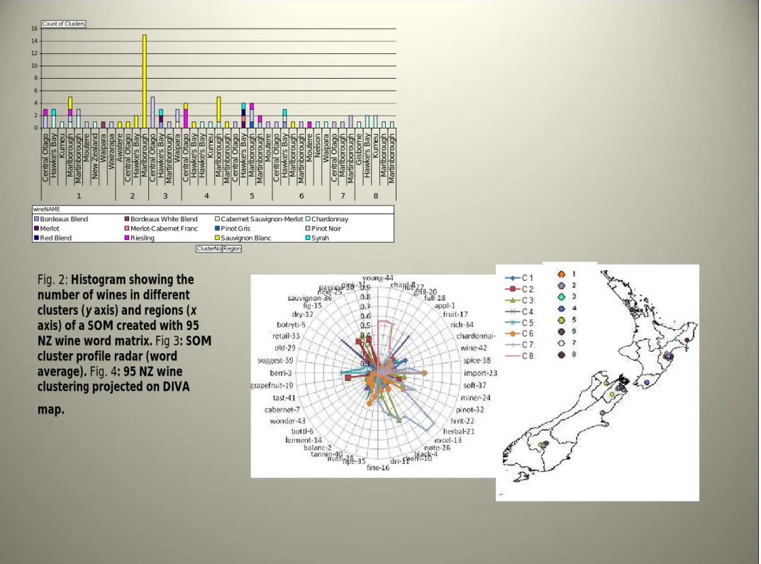
Fig. 2: Histogram showing the

number of wines in different

clusters (y axis) and regions (x

axis) of a SOM created with 95

NZ wine word matrix. Fig 3: SOM

cluster profile radar (word

average). Fig. 4: 95 NZ wine

clustering projected on DIVA

map.

(41)

2 R e d Ble nd H a w ke 's Ba y 2 9 Pino t N o ir Ma rtin b oro u gh Merlo t-C a b e rn e t Fra n c H aw ke 's Bay 2 8 Pin ot N o ir Marlb oro u gh Pin o t N o ir Marlb o ro u g h 5 Me rlo t H aw ke's Ba y R ies lin g Martin b oro ug h 7 4 R ies lin g Ma rlb o rou g h 71 R ie s lin g C e n tra l Ota g o Sa uvign o n Bla n c C en tral Otag o 1 3 Sa uvign o n Bla n c Ma rtinb o ro u g h R ie s lin g C en tra l Ota go 8 9 Sa u vig no n Bla n c Marlb o ro u gh 5 2 C h ard o nn a y Ma rlb o ro u g h 7 3 R ies lin g C e ntra l Ota go 25 Pin o t N o ir C e n tra l Ota g o 40 Syra h H a w ke 's Ba y 5 6 Pin o t Gris Marlb o ro u gh 48 C h a rd o n na y Kum eu 7 7

Sau vign o n Bla nc H a w ke 's Ba y 1 2 Sa u vig no n Bla n c Marlb oro u gh 4 6 C h a rd o n na y H a w ke 's Ba y 5 0 C h a rd o n na y Ku m eu 5 1 C h a rd o n na y Ma rlb o rou g h 1 6

C a be rne t Sau vig n o n-Me rlo t Wa ipa ra 9 R ies lin g Ma rlb o rou g h 31 Pin o t N o ir Martin b oro ug h 3 5 Sa uvign o n Bla n c Ma rlb oro ug h 8 5 Sa u vig no n Bla n c Marlb o ro u gh 4 9 C h ard o nn a y Ku m eu 59 Pin o t N o ir C e n tra l Ota g o 64 Pin o t N o ir C e n tra l Ota g o 68 Pin o t N o ir Wa ip a ra 5 8 Pin o t N oir C en tra l Ota go 6 5 Pin o t N oir Marlb o ro u gh 6 7 Pin o t N o ir Mou te re 88

Sau vig n o n Bla nc Ma rlbo rou g h 1 7 C h ard on n a y H aw ke's Bay 4 C h a rd o n na y Martin b oro ug h 4 4 C h a rd o n na y Gis b orn e 4 7 C h a rd o n na y H a w ke 's Ba y 4 3 Bo rd e a ux Ble n d H a w ke 's Ba y 8 Pino t N o ir Ma rtin b oro u gh 5 7 Pin o t N o ir C en tra l Ota go 4 1 Syrah H a w ke 's Ba y 37

Sau vign o n Bla nc Ma rlbo ro ug h

70 Pin o t N o ir Waira ra p a

1 5

Bord ea u x Wh ite Blen d Wa ip a ra Va lle y 5 3 C h ard on n a y Ma rtinb o rou g h 5 4 C h ard on n a y N e w Ze ala n d 1 9 C h ard o nn a y Ku m eu 2 0 C h ard o nn a y Ma rlb o ro u g h 26 Pin o t N o ir C e n tra l Ota g o 69 Pin o t N o ir Wa ip a ra 6 1 Pin o t N oir C en tra l Ota go 6 0 Pin o t N o ir C e ntra l Ota go 21 C h a rd o n na y Martin b oro ug h 1 8 C h a rd o n na y H a w ke 's Ba y 3 2 R ies lin g C e n tra l Ota g o 4 2 Syra h H a w ke 's Ba y 2 3 Me rlot H aw ke 's Bay 3 8 Sa uvign o n Bla n c Ma rlb oro ug h 9 2 Sa u vig no n Bla n c Marlb o ro u gh 7 5 Sa u vig n on Blan c Aw a te re Va lley 8 0 Sa u vig n on Blan c Ma rlb o ro u g h 8 6 Sa u vig n on Blan c Ma rlb o ro u g h 62 Pin o t N o ir C e n tra l Ota g o 66 Pin o t N o ir Ma rlbo ro ug h 7 Pin o t N o ir Martin b oro ug h 1 4 Bord ea u x Ble nd H a w ke's Ba y 3 4

Sau vign o n Bla nc Ma rlbo ro ug h

7 9

Sau vign o n Bla nc H a w ke 's Ba y 3 9 Sa u vig no n Bla n c Marlb oro u gh 8 2 Sa u vig n on Bla n c Marlb o ro u g h 7 8

Sau vig n o n Blan c H a w ke 's Ba y

9 3

Sau vig n o n Blan c Ma rlb o rou g h 3 0 Pino t N o ir Ma rtin b oro u gh 3 3 R ie s lin g Mo u te re 6 3 Pin ot N o ir C en tral Otag o 5 5 C h ard on n a y Wa ip a ra 6 Pin o t N o ir

Martin b oro ug h Terra ce 2 2 C h a rd o n na y N e ls on 4 5 C h a rd o n na y 83

Sau vign o n Bla nc Ma rlbo ro ug h 7 6 Sa uvign o n Bla n c C en tral Otag o 8 1 Sa uvign o n Bla n c Ma rlb oro ug h 9 1 Sa u vig no n Bla n c Marlb o ro u gh 3 6 Sa u vig n on Blan c Ma rlb o ro u g h 8 7 Sa u vig n on Blan c Ma rlb o ro u g h

Three cluster SOM created with 44 weights calculated by applying the (

tf x idf

)

formula to words occurring more than twice in the taster comments of 95 wines

(42)

appl-1

0.00

0.76 berri-3

0.00

0.86 black-4

0.00

0.72 cherri-10

0.00

0.59 grapefruit-19

0.00

0.71 herbal-21

0.00

0.98 nut-27

0.00

0.59 nutti-28

0.00

0.88 passion-30

0.00

0.83 pink-31

0.00

0.51 tannin-40

0.00

0.67 old-29

0.00

0.56 A few SOM components showing the word weights in the

clustering

(43)

0 2 4 6 8 10 12 14 16

C

e

n

tr

a

l

O

ta

g

o

H

a

w

k

e

's

B

a

y

K

u

m

e

u

M

a

rl

b

o

ro

u

g

h

M

a

rt

in

b

o

ro

u

g

h

M

o

u

te

re

N

e

w

Z

e

a

la

n

d

W

a

ip

a

ra

W

a

ir

a

ra

p

a

A

w

a

te

re

C

e

n

tr

a

l

O

ta

g

o

H

a

w

k

e

's

B

a

y

M

a

rl

b

o

ro

u

g

h

C

e

n

tr

a

l

O

ta

g

o

H

a

w

k

e

's

B

a

y

M

a

rt

in

b

o

ro

u

g

h

W

a

ip

a

ra

C

e

n

tr

a

l

O

ta

g

o

H

a

w

k

e

's

B

a

y

H

a

w

k

e

's

B

a

y

K

u

m

e

u

M

a

rl

b

o

ro

u

g

h

M

a

rt

in

b

o

ro

u

g

h

C

e

n

tr

a

l

O

ta

g

o

H

a

w

k

e

's

B

a

y

M

a

rl

b

o

ro

u

g

h

M

a

rt

in

b

o

ro

u

g

h

M

o

u

te

re

C

e

n

tr

a

l

O

ta

g

o

H

a

w

k

e

's

B

a

y

M

a

rl

b

o

ro

u

g

h

M

a

rt

in

b

o

ro

u

g

h

M

o

u

te

re

N

e

ls

o

n

W

a

ip

a

ra

C

e

n

tr

a

l

O

ta

g

o

M

a

rl

b

o

ro

u

g

h

M

a

rt

in

b

o

ro

u

g

h

G

is

b

o

rn

e

H

a

w

k

e

's

B

a

y

K

u

m

e

u

M

a

rl

b

o

ro

u

g

h

M

a

rt

in

b

o

ro

u

g

h

1

2

3

4

5

6

7

8

Bordeaux Blend Bordeaux White Blend Cabernet Sauvignon-Merlot Chardonnay Merlot Merlot-Cabernet Franc Pinot Gris Pinot Noir Red Blend Riesling Sauvignon Blanc Syrah

Count of Clusters

ClusterNo Region wineNAME

Graph showing the wine grouping of the 8 cluster SOM of wine

taster comments. The clustering reflects the

wine variety by region.

For example, Cluster 2 has

Sauvignon Blanc

from Awatere, Central

Otago, Hawke’s Bay and Marlborough regions

(44)

Sensors

A variety of climate, atmospheric, soil and plant sensors to

collect growth influence factors

(45)

An integrated multi-function sensor

Climate (wind, rain/precipitation,

humidity, pressure, sunlight),

cloud cover

Atmosphere (carbon density,

herbicide saturation)

Radiation (UV, haze

effect etc)

Terrain and Soil (type,

moisture, temp)

Plant (roots, vine, leaves, grapes)

Precision data examples:

• Determining dew-point

• Measuring sap rise

• Correlating soil moisture/temp

with radiation levels

and atmospheric pressure

…

Prediction

algorithms for frost

and irrigation

(46)

Wireless

…

Geo-computational topology for analysing logged data

Data logger upload to central computer

Pseudo-real time ftp

connection...packets at 30

sec intervals

Statistics, correlations

and trend analysis

(47)

(48)

(49)

Soil moisture

measurement for

(50)

Image Processing and Resistence based

methods

(51)

Image Processing with probe & infra-red

methods

(52)

Image Processing and Solar Intensity

(lux)

(cloud formations)

• Time interval photos of sky

• Classification of cloud cover (full, partial, clear)

(53)

All of the polymer films on a set of electrodes (sensors) start out at

a measured resistance, their

baseline resistance

. If there has been

no change in the composition of the air, the films stay at the

baseline resistance and the percent change is zero

e- _e- _e- _e- _e- _e

-The Electronic Nose

Measuring odour as a test of grape quality

using Baseline Resistance

(54)

If a different compound had caused the air to change, the pattern of the

polymer films' change would have been different:

Basic Concept - each polymer changes its size, and therefore its resistance, by

a different amount, making a pattern of the change. Known odour spectrum for

grapes compared with observed (sampled) odours.

Odour – The Electronic Nose

e- e- e -e- e -e -e -e -e -e -e- e

(55)

-Speech Processing

and

(56)

(57)

Sommelier Voice Printing

…

English

Spanish

French

(58)

Eno-Humanas Conclusions

…

Historical data

Chemistry

Expert input

Consumers

Multivariate

complexity

Indefinite

prediction

potential

Plot discrete

values and

determine their

dependencies

Neural

Network

technologies

Prediction

potential

increases

Time Series

experiments

with lots of

data required!

(59)

In our start up phase…..

Mostly identifying variables, gathering data

and conducting multivariate analysis for

cross correlating dependencies and other

intrinsic data relationships.

(60)