Impact of diagonal cumulation rule on FTA
utilization : evidence from bilateral and
multilateral FTAs between Japan and Thailand
著者
Hayakawa Kazunobu
権利
Copyrights 日本貿易振興機構(ジェトロ)アジア
経済研究所 / Institute of Developing
Economies, Japan External Trade Organization
(IDE-JETRO) http://www.ide.go.jp
journal or
publication title
IDE Discussion Paper
volume
372
year
2012-11-01
Abstract
In this paper, we empirically investigate the effect of diagonal cumulation on free trade agreement (FTA) utilization by exploring Thai exports to Japan under two kinds of FTA schemes. While the one scheme adopts bilateral cumulation, the other scheme does diagonal cumulation. Comparing trade under these two kinds of FTAs, we can examine the effect of diagonal cumulation without relying on not only the variation in cumulation rules across country pairs but also the variation across years. In short, our estimates do not suffer from biases from time-variant elements and country pair-specific elements. As a result, our estimates show around 4% trade creation effect of diagonal cumulation, which is much smaller than the estimates in the previous studies (around 15%).
INSTITUTE OF DEVELOPING ECONOMIES
IDE Discussion Papers are preliminary materials circulated to stimulate discussions and critical comments
Keywords: FTA; diagonal cumulation; trade creation effect JEL classification: F15; F23
#
Author. Kazunobu Hayakawa, Bangkok Research Center, Japan External Trade Organization, 16th Floor, Nantawan Building, 161 Rajadamri Road, Pathumwan, Bangkok 10330, Thailand. Tel: 66-2-253-6441; Fax: 66-2-254-1447. E-mail: [email protected].
IDE DISCUSSION PAPER No. 372
Impact of Diagonal Cumulation Rule on FTA
Utilization: Evidence from Bilateral and
Multilateral FTAs between Japan and Thailand
Kazunobu HAYAKAWA#The Institute of Developing Economies (IDE) is a semigovernmental, nonpartisan, nonprofit research institute, founded in 1958. The Institute merged with the Japan External Trade Organization (JETRO) on July 1, 1998. The Institute conducts basic and comprehensive studies on economic and related affairs in all developing countries and regions, including Asia, the Middle East, Africa, Latin America, Oceania, and Eastern Europe.
The views expressed in this publication are those of the author(s). Publication does not imply endorsement by the Institute of Developing Economies of any of the views expressed within.
INSTITUTE OF DEVELOPING ECONOMIES (IDE), JETRO 3-2-2, WAKABA,MIHAMA-KU,CHIBA-SHI
CHIBA 261-8545, JAPAN
©2012 by Institute of Developing Economies, JETRO
No part of this publication may be reproduced without the prior permission of the IDE-JETRO.
1
Impact of Diagonal Cumulation Rule on FTA Utilization:
Evidence from Bilateral and Multilateral FTAs between
Japan and Thailand
Kazunobu HAYAKAWA#§
Bangkok Research Center, Japan External Trade Organization, Thailand
Abstract: In this paper, we empirically investigate the effect of diagonal cumulation on free trade agreement (FTA) utilization by exploring Thai exports to Japan under two kinds of FTA schemes. While the one scheme adopts bilateral cumulation, the other scheme does diagonal cumulation. Comparing trade under these two kinds of FTAs, we can examine the effect of diagonal cumulation without relying on not only the variation in cumulation rules across country pairs but also the variation across years. In short, our estimates do not suffer from biases from time-variant elements and country pair-specific elements. As a result, our estimates show around 4% trade creation effect of diagonal cumulation, which is much smaller than the estimates in the previous studies (around 15%).
Keywords: FTA; diagonal cumulation; trade creation effect JEL Classification: F15; F23
#
Author. Kazunobu Hayakawa, Bangkok Research Center, Japan External Trade Organization, 16th Floor, Nantawan Building, 161 Rajadamri Road, Pathumwan, Bangkok 10330, Thailand. Tel: 66-2-253-6441; Fax: 66-2-254-1447. E-mail: [email protected].
§
I am grateful to Archanun Kohpaiboon for providing me with the data used in this study. I also would like to thank Fukunari Kimura, Toshihiro Okubo, Taiyo Yoshimi, Wisarn Pupphavesa and seminar participants in Keio University, Nanzan University, and Thailand Development Research Institute for their helpful comments. The opinions expressed in this paper are those of the author and do not represent the views of any of the institutions with which I am affiliated.
2
1. Introduction
Allowing “diagonal cumulation” is a potential advantage of multilateral or region-wide free trade agreements (FTAs) over bilateral FTAs. In the bilateral cumulation, which applies to bilateral FTAs, materials originating in one country could be considered as those originating in the partner country and vice versa. On the other hand, the diagonal cumulation applies to FTAs among more than two countries. In the diagonal cumulation, materials originating in one country could be considered as those originating in all of the FTA partner countries. Namely, this enables FTA users to cumulate the value of intermediates from not only the exporting country but also other member countries in determining originating status on the products to be exported. It is also worth noting full cumulation, which is more flexible than the diagonal cumulation and allows FTA users to cumulate all materials used in the preferential area. In some multilateral FTAs, this rule of diagonal cumulation in addition to full cumulation has been adopted (for more details, see, for example, Augier et al., 2005).
Without the diagonal cumulation provision, the multilateral FTA is not different from “multiple” bilateral FTAs and is unable to realize their potential advantages. Namely, in this case, a multilateral FTA among countries A, B, and C is qualitatively not so different from three bilateral FTAs between countries A and B, between countries B and C, and between countries A and C. Such a multilateral FTA still has some advantages such as common product specific rules of origin (ROOs), which reduce transaction costs for the use of FTA schemes in exporting to multiple member countries simultaneously. However, without the diagonal cumulation provision, when a firm in country B exports to country A, that firm cannot obtain originating status for inputs from country C. Particularly in the recent era when international production networks have developed, the cumulation of such inputs from country C sometimes becomes critical in complying with the ROOs. The cumulation of such inputs from the other member countries enables firms to comply more easily with the ROOs. As a result, FTAs with diagonal cumulation are expected to have larger trade creation effects than FTAs with bilateral cumulation.
In the academic field, some studies try to quantify the trade creation effect of diagonal cumulation (Augier et al., 2005; Estevadeordal and Suominen, 2008; Innwon and Soonchan, 2009). All of these studies extend the gravity equation by introducing FTA dummy variables, which are differentiated according to cumulation types, including full cumulation, diagonal cumulation, and bilateral cumulation. Estevadeordal and Suominen (2008) examines bilateral trade flow among 155 countries during the 1981-2001 period and finds that members in the full cumulation FTA trade 109% more
3
than those in the bilateral cumulation FTA. In Innwon and Soonchan (2009), the trade flow among 154 countries during 1980-2005 is investigated. The major finding is that full cumulation, diagonal cumulation, and bilateral cumulation increase bilateral trade values by 35.8%, 16.0%, and 0.9% (insignificant), respectively. Augier et al. (2005) examines bilateral trade flow among 38 countries in 1995 and 1999 and finds that the introduction of diagonal cumulation increases trade by 7.4%-22.1%. In sum, we may conclude that the diagonal cumulation increases trade by around 15%.
In particular, Augier et al. (2005) is the study that most carefully examines the trade creation effect of diagonal cumulation. It focuses on the effect within the pan-European system of diagonal cumulation (PECS), which is the principal form of diagonal cumulation between the European Union (EU) and its partner countries. The PECS came into force in 1997 with a group of EU partner countries (CEFTA, EFTA, and the Baltic states). Namely, the “cumulatable” area expanded in 1997. By using this geographical expansion as a natural experiment, authors quantify the trade creation effect of diagonal cumulation. Thus, unlike the two other studies, Augier et al. (2005) does not rely on the variation across country pairs (i.e. differences between trade in the members of FTA with diagonal cumulation and trade in those of FTA without it) by comparing trade flow in the same country pair before and after the introduction of diagonal cumulation. Indeed, if FTAs with the diagonal cumulation provision are more likely to have other special elements for trade creation compared with FTAs with only the bilateral cumulation, then the estimates in the two other studies capture not only the effect of diagonal cumulation but also the effects of those special elements. In other words, the estimate in Augier et al. (2005) shows the purer magnitude of the trade creation effect of diagonal cumulation.
Against this backdrop, we empirically investigate the trade creation effect of diagonal cumulation for another case as a natural experiment. Specifically, this paper explores the FTA utilization in Thai exports to Japan. One unique point in this trade flow is that two kinds of FTA schemes are available, one of which adopts bilateral cumulation and another of which does diagonal cumulation. The Japan-Thailand Economic Partnership Agreement (JTEPA) is a bilateral FTA between Thailand and Japan that entered into force in November 2007. On the other hand, the ASEAN-Japan Comprehensive Economic Partnership (AJCEP) is a multilateral FTA of Japan with ASEAN countries, including Thailand. It entered into force during December 2008 in Japan and during June 2009 in Thailand. One of the important differences between JTEPA and AJCEP is the type of cumulation. JTEPA adopts bilateral cumulation, while AJCEP accepts diagonal cumulation and thus allows users to cumulate inputs from all
4
member countries. Namely, AJCEP has an advantage in terms of the cumulation type. Thus, by exploiting differences between preferential trade under AJCEP and JTEPA, this paper tries to quantify the effect of diagonal cumulation.
More specifically, this paper examines the effect of diagonal cumulation on FTA utilization rather than that on total trade values (including not only those under FTA schemes but also those under MFN scheme). In the academic field, there are several papers analyzing the determinants on the utilization of preferential rates. Bureau et al. (2007) examines utilization of the Generalized System of Preferences (GSP) granted by the EU and the United States to developing countries in the agri-goods sector, while Cadot et al. (2006) focuses on the trade of the EU and the United States with their preferential trading partners. Francois et al. (2006) and Manchin (2006) examine the preferential trade relations of the EU and non-least-developed African, Caribbean, and Pacific (ACP) countries under the Cotonou Agreement, while Hakobyan (2010) examines U.S. GSP utilization by 143 GSP eligible countries. The elements examined for the determinants on utilization of preferential rates in those studies are almost identical, particularly tariff margin (i.e. difference between MFN rates and preferential rates) and restrictiveness of ROOs. This is the first paper that examines the effect of diagonal cumulation provision in addition to tariff margin and ROOs on FTA utilization. Our strategy for identifying the effect of diagonal cumulation has the following advantages compared with the cases of the above-mentioned previous studies. As in Augier et al. (2005), we do not rely on the variation across country pairs because of our focus on Thai exports to Japan. Furthermore, unlike Augier et al. (2005), we do not rely on the variation in trade across years (i.e. differences in trade between years before and after the introduction of diagonal cumulation) due to our analysis for single year (i.e., 2010). This is possible because we can compare trade in a country pair under FTA with diagonal cumulation with trade in the same pair under FTA without diagonal cumulation. Although Augier et al. (2005) tries to control for the other time-variant elements by introducing many observables into the equation, its estimates may still surfer from biases by unobservable time-variant elements. As a result, our estimate will show a purer effect of diagonal cumulation than the estimates in the previous studies.
The rest of this paper is organized as follows. The next section provides the general information on JTEPA and AJCEP, including the level of preferential rates, ROOs, and so on. After explaining our empirical method in Section 3, we report the empirical results on the effect of diagonal cumulation on FTA utilization rates in Section 4. Last, Section 5 concludes on this paper.
5
2. JTEPA and AJCEP
This section presents some basic information on JTEPA and AJCEP. JTEPA is a bilateral FTA between Thailand and Japan, entered into force in November 2007. In addition to the liberalization of trade in goods and services, this agreement includes various provisions on mutual recognition, movement of natural persons, intellectual property, government procurement, and so on. On the other hand, AJCEP is a multilateral FTA of Japan with ASEAN countries. For Japan, AJCEP is the first multilateral FTA. It was entered into force in December 2008 in Japan, Singapore, Vietnam, Laos, and Myanmar. In 2009, it entered into force in Brunei, Malaysia, Thailand, and Cambodia, in addition to the Philippines in 2010. Thus, as of June 2012, Indonesia was the only country in which AJCEP was not entered into force. As mentioned in the introductory section, while JTEPA adopts bilateral cumulation, the diagonal cumulation rule is available in AJCEP, which is referred in “Accumulation” in Article 29 in the legal text of AJCEP.
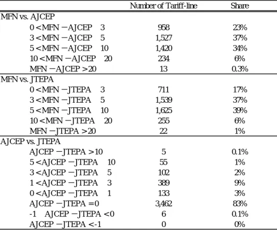
We first take an overview of preferential tariff rates. Table 1 compares three kinds of tariff rates in Japan for products from Thailand in 2010, MFN rates, AJCEP preferential rates, and JTEPA preferential rates. The comparison is conducted at the tariff-line level, i.e. the Harmonized System (HS) 2007 9-digit level. The data are from the World Integrated Trade Solution Database, particularly TRAINS raw data.1 In this table, products are restricted only to those having both AJCEP rates and JTEPA rates, which are 4,152 products.2 AJCEP rates and JTEPA rates are available for 4,311 and 4,294 products in 2010, respectively. Namely, the coverage of preferential products is almost common between AJCEP and JTEPA. Also, the tariff line includes 9,025 products in HS2007, so that nearly half of all products are examined here.
=== Table 1 ===
There are two noteworthy points. Firstly, a major range of tariff margin against MFN rates in both AJCEP and JTEPA schemes is 3-10%. In both schemes, around 70% of preferential products fall into this range. Several studies on the estimates of the tariff equivalent of fixed costs for FTA use reveal that those lie between 3% and 5%.3 Thus,
1
http://wits.worldbank.org/wits/
2
Also, we drop products in which MFN rates are specific tariff rates.
3
Cadot and de Melo (2007) concludes that such fixed costs range between 3% and 5% of final product prices. Francois et al. (2006) applies the threshold regression approach, which was developed by Hansen (2000), to the utilization rate of Cotonou preferences and finds their range to
6
AJCEP and JTEPA have tariff margin sufficient to cover fixed costs for those used. Secondly, only six products have lower preferential rates in AJCEP than in JTEPA. This is because both JTEPA and AJCEP take a style of gradual tariff elimination and further because, as mentioned above, JTEPA entered into force earlier than AJCEP. However, almost all products (83%) have the same level of preferential rates between AJCEP and JTEPA in 2010. Moreover, 96% of all products have as low as or lower than a 3% difference in preferential rates.
Next, Table 2 shows the matrix of ROOs between AJCEP and JTEPA. In the legal texts of agreements, ROOs are defined at the HS2002 6-digit level. In this table, products are again restricted only to those having both AJCEP rates and JTEPA rates, which are 2,199 products at the HS2002 6-digit level. Specifically, we classify ROOs into 14 types: CC, CC/RVC, CC&TECH, CH, CH/RVC, CH/TECH, CH/RVC/TECH, CH&RVC, CH&TECH, CS, CS/RVC, CS/RVC/TECH, RVC, and WO. “CS”, “CH”, and “CC” are the ROO criteria of “Change in Subheading”, “Change in Heading”, and “Change in Chapter”, respectively. “WO” indicates wholly-obtained criterion. “RVC” is the ROO criteria of the less than 40% real value-added content. “TECH” is the specific manufacturing or processing operations criterion. Some products require meeting both (&) or either (/) two or three kinds of criteria. Three points are to be noted in Table 2. Firstly, 50% of products have common ROO types between AJCEP and JTEPA. In other words, in 50% of products, different ROO types are strategically or selectively set between AJCEP and JTEPA. Secondly, while the major rule in AJCEP is CH/RVC (i.e. the rule not listed in Product Specific Rule), that in JTEPA is CC. Generally, it becomes severe in the order of CC, CH, and CS. Also, the criteria combined by AND (&) becomes severer than those combined by OR (/). Thus, we may say that JTEPA adopts the severer ROOs than AJCEP. Thirdly, compared with the case of AJCEP, ROOs in the case of AJCEP are more diverged.
=== Table 2 ===
Last, we take an overview of FTA utilization rates in AJCEP and JTEPA. For example, AJCEP utilization rates are calculated as the share of exports under the AJCEP scheme in total exports in all products with AJCEP preferential rates. The data on Thai exports to Japan under AJCEP and JTEPA schemes are available by the Bureau of Trade Preference Development, Department of Foreign Trade, Ministry of Commerce. The be between 4% and 4.5%. Employing the threshold regression method for all existing FTAs in the world, Hayakawa (2011) estimates those costs to be around 3%.
7
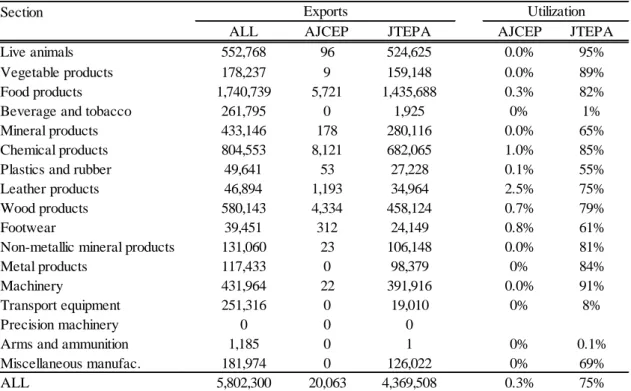
data are provided at the HS2007 6-digit level. We also obtain the data on total exports, including exports under the MFN scheme from UN Comtrade (United Nations). In Table 3, the utilization rates are reported by section. In the calculation, the denominator is total exports in only products with preferential rates in each section. In Table 3, in total, we can see outstandingly low utilization rates of AJCEP (0.3%). Since those of JTEPA have 75% in total, most of the exports (in products with preferential rates) are conducted under JTEPA rather than MFN or AJCEP. Particularly in live animals and machinery products, more than 90% of products are exported to Japan under the JTEPA scheme. The relatively high (but absolutely low) rates can be observed in leather products in the case of AJCEP.
=== Table 3 ===
3. Empirical Framework
In this section, we present our empirical framework to analyze the effect of diagonal cumulation on FTA utilization. To do that, we examine the determinants of FTA utilization rates for AJCEP and JTEPA. In specifying our model, the theoretical framework provided by Demidova and Krishna (2008), which introduces firm heterogeneity in terms of productivity into firms’ choices on tariff schemes, will be useful. It theoretically examines what kinds of firms are more likely to use the FTA scheme rather than the MFN scheme. Here, we focus on exporters’ decisions on FTA use because, in using FTA schemes in importing, firms just need to submit the certificates of origin prepared by exporting firms to customs. Namely, importers always prefer the use of an FTA if exporters afford using FTA schemes. Thus, in order to highlight the economically meaningful decision making, we consider the exporters’ decisions on FTA use.
The use of FTA schemes in exporting is dependent upon its benefit and cost. The benefit is how much firms can save on their tariff payment by using FTA preferential rates. If firms choose to use an FTA scheme, then they can export their products with the FTA preferential tariff rates. Otherwise, they must pay the general tariff rates, which are mainly MFN rates. Therefore, the larger difference between FTA rates and MFN rates leads to a larger amount of tariff payment saving. In other words, the larger the tariff margin (difference between preferential and general tariff rates), the more likely the firms are to use FTA schemes. The other important element is the size of exports because the use of FTA schemes for the larger size of exports leads to a bigger reduction
8
of tariff payment. Therefore, for example, firms’ higher productivity plays a role of increasing the reduction of tariff payment. In other words, differences in productivity distribution across industries also lead to the differences in industry-level FTA utilization.
On the other hand, the cost of FTA utilization is “procurement adjustment cost”. For the use of an FTA scheme, firms need to secure the ROOs of their product. Complying with the ROO requirement may force firms to change procurement origins and raise their procurement costs since the original ones should be optimal.4 Thus, the unit cost in the case of an FTA is as high as or higher than that in the case of general rates. The difference in unit costs will depend on how restrictive the ROOs are for firms. In other words, the less restrictive the ROOs, the more likely the firms are to use FTA schemes in their exporting. In addition, for the use of FTA rates, firms have to incur a certain level of fixed costs. For example, in order to secure ROOs, exporters must collect several kinds of documents, including a list of inputs, production flow chart, production instructions, invoices for each input, contract document, and so on. Based on these documents, exporters apply certificates of origin to the authority. These works become non-negligible costs for exporters. Obviously, the lower fixed costs for FTA use encourage firms to use FTA schemes.
Against this framework, our model becomes more complicated because we need to consider not only the choice between MFN rates and FTA rates but also that between AJCEP rates and JTEPA rates. In this paper, we consider what kinds of elements affect the choice between the use of AJCEP and that of JTEPA, under the condition of firms’ choosing the use of FTA schemes over the use of the MFN scheme. Obviously, the AJCEP scheme is more likely to be used than the JTEPA scheme if AJCEP preferential rates are lower than JTEPA preferential rates or if ROOs in AJCEP are less restrictive than those in JTEPA. Furthermore, allowing the cumulation of inputs from the other FTA member countries enables firms to comply more easily with the ROOs. Namely, the provision of diagonal cumulation in AJCEP plays the role of reducing procurement adjustment costs, resulting in the more likely use of the AJCEP scheme.
As a result, we specify our empirical model as a Heckman model. The choice of preferential tariff schemes between AJCEP and JTEPA, i.e. outcome, is examined by estimating:
𝑌𝑝𝐴𝐴𝐴𝐴𝐴
𝑌𝑝𝐴𝐽𝐴𝐴𝐴 = 𝐳𝑝𝛄 + 𝑣𝑝. (1)
4
The inputs from the FTA member countries may become cheaper because of importing under preferential tariff rates, not general tariff rates.
9
Ysp indicates exports from Thailand to Japan in product p under FTA scheme s. A vector of z includes the above-mentioned elements that affect the choice of preferential tariff schemes between AJCEP and JTEPA. A vector of γ is coefficients to be estimated. The dependent variable for product p is observed if:
max 𝑖∈𝑁𝑝{𝜋𝑖 𝐹𝐹𝐹− 𝜋 𝑖𝑀𝐹𝑁} = max𝑖∈𝑁 𝑝�max�𝜋𝑖 𝐹𝐴𝐴𝐴𝐴, 𝜋 𝑖𝐴𝐹𝐴𝐴𝐹� − 𝜋𝑖𝑀𝐹𝑁� = 𝐱𝑝𝛃 + 𝑢𝑝 > 0. (2)
This is called selection equation. πis is firm i’s profits from exporting from Thailand to Japan under tariff scheme s. Np is a set of firms producing product p. Namely, the selection equation describes whether or not at least one firm obtains the larger profits from exporting under the FTA scheme than from exporting under the MFN scheme. A vector of x includes the above-mentioned elements that affect the choice between the use of the FTA scheme and that of the MFN scheme. A vector of β is coefficients to be estimated. The residuals in these two equations are assumed to follow:
𝑢~𝑁(0,1), 𝑣~𝑁(0, 𝜎2), corr(𝑢, 𝑣) = 𝜌.
σ is the standard error of the residual in the outcome equation. ρ is a parameter to be estimated. We will estimate this model by the maximum likelihood estimation technique.
Based on the above discussion, the elements of z are as follows. The first element is the difference between AJCEP and JTEPA preferential rates, which is given by
(tpAJCEP − tpJETPA), where tps is preferential tariff rates (%) in product p under FTA
scheme s. The second one is the difference in the restrictiveness of ROO types between AJCEP and JTEPA. In the literature, a quantitative measure of restrictiveness on ROOs has been proposed. The restrictive index proposed in Estevadeordal (2000) and Estevadeordal and Suominen (2004) ranges from minimum 1 (least restrictive) to maximum 7 (most restrictive) by ROOs category. These papers score ROOs in FTAs in the United States and Europe. For example, a lower restrictiveness score is given for RVC than for CC. Following their ways (with a bit of modification), we assign scores to each type of ROO and introduce that as an independent variable, (ROOpAJCEP −
ROOpJETPA), where ROOps is the restrictiveness of ROOs in product p under FTA scheme
s. The score of each ROO type in this paper is listed in the Appendix.
Under the controlling of these differences in preferential rates and ROOs, the effects of the remaining differences between AJCEP and JTEPA will appear in the estimate of a constant term. The most important difference is the provision of the diagonal cumulation rule in AJCEP. Basically, there seems to be no other outstanding differences between AJCEP and JTEPA. Thus, the major components in the constant
10
term will show the effect of the diagonal cumulation rule. In particular, the formulation of our dependent variable in equation (1) is the ratio of exports under AJCEP to those under JTEPA, so that the estimates of the constant term could be directly interpreted as indicating the magnitude of the trade creation effect of the diagonal cumulation rule.5 Compared with the elements of z, it is difficult to construct the elements of x. We first need to control for the difference between FTA preferential rates and MFN rates, which is often called the tariff margin. However, two kinds of FTA preferential rates are available. We try two kinds of measures on the tariff margin. While the one is the difference of MFN rates with the lower rates between AJCEP rates and JTEPA rates, the other is that with the average rates between AJCEP rates and JTEPA rates. Specifically, the former measure is (tpMFN – min{tpAJCEP, tpJETPA}) and the latter one is (tpMFN –
{(tpAJCEP+ tpJETPA)/2}). Secondly, it is necessary to control for the restrictiveness of
ROOs. As well as the case of the tariff margin, we include two kinds of restrictive measures. While the one is the less restrictive score of ROOs between AJCEP schemes and JTEPA schemes, the other is the average score of ROOs between AJCEP schemes and JTEPA schemes. Specifically, the former measure is (min{ROOpAJCEP, ROOpJETPA}) and the latter one is ((ROOpAJCEP+ ROOpJETPA)/2). Lastly, we control for the differences in firms’ productivity distribution across products. To do that, we introduce the Revealed Comparative Advantage (RCA) Index for Thailand. Specifically, it is calculated for product p as [(Thai exports of product p to the world / Thai total exports to the world) / (World exports of product p / World total exports)]. The larger index means a larger comparative advantage or more international competitiveness. The difference in international competitiveness across products will be associated with that in firms’ productivity distribution across products.
The data sources are basically the same as in the previous section. The data for calculating the RCA Index are obtained from the UN Comtrade. It is worth noting how to aggregate the tariff data. The original data source provides us the data on tariff rates at the tariff-line level in HS2007, i.e. the HS2007 9-digit level. On the other hand, ROOs are defined at the 6-digit level in HS2002. The conversion table between HS2002 and HS2007 is available at the 6-digit level,6 so that we decide to aggregate and convert tariff data in the HS2007 9-digit level to those in the HS2002 6-digit level. We
5
In this formulation, the products with zero exports under JTEPA are automatically dropped from the sample in the outcome equation. However, the number of such products is only five, which together account for only 0.2% of all observations.
6
http://unstats.un.org/unsd/trade/conversions/HS%20Correlation%20and%20Conversion%20tables.ht m
11
adopt two kinds of aggregation from the 9-digit level to 6-digit. One is to take a simple average of 9-digit level tariff rates in each 6-digit level. The other is to use the lowest rates in each 6-digit level. As a result, we obtain two kinds of tariff rates at the 6-digit level in HS2007. Then, these tariff rates are converted to the version of HS2002. In doing that, one product in HS2007 may be corresponding to multiple products in HS2002. Then, we take a simple average.
4. Empirical Results
This section reports our estimation results. Basic statistics are reported in Table 4. For example, taking a look at the HS 6-digit level, we can see that there are products in which exports under AJCEP are around five times as large as those under JTEPA (see maximum values in a dependent variable in the outcome equation). Table 5 shows our baseline results. Columns (I) and (III) use tariff rates based on the mean of tariff rates at the 9-digit level while columns (II) and (IV) do those based on the minimum rates at the 9-digit level (see the previous section). Also, in the selection equation, columns (I) and (II) use the lower tariff margin with MFN rates between cases of AJCEP and JTEPA and the less restrictive score of ROOs between those cases. Columns (III) and (IV) do the average tariff margin with MFN rates and the average restrictive score of ROOs. All estimations show the significant results in Rho (ρ), indicating the existence of selection mechanics in equation (1).
=== Tables 4 & 5 ===
The results in the selection equation are as follows. Firstly, as is consistent with our expectation, coefficients for MFN Margin are estimated to be significantly positive, implying that products with the larger tariff margin with MFN rates are more likely to be exported under FTA schemes. Such a positive role of the tariff margin in the use of the FTA scheme is a common result in this literature. Secondly, the ROO Restrictive Index has positively significant coefficients. The products with the less restrictive ROOs are expected to be exported under the FTA scheme, so that such a positive coefficient is not consistent with this expectation. This result may indicate that the way of scoring ROOs used in the previous studies is not appropriate in the context of AJCEP and JTEPA. Lastly, the coefficients for the RCA Index are estimated to be significantly positive, indicating that products with more international competitiveness are more likely to be exported under the FTA scheme. Such products have larger exports,
12
resulting in a larger reduction of tariff payment through the use of the FTA scheme. On the other hand, the results in the outcome equation are the following. While the coefficients for the preferential margin are insignificantly estimated, those for ROO Difference are insignificant or positive at a 10% significance level. The former results may indicate at least that the choice of preferential tariff schemes is not linearly related to the difference in the level of those preferential rates. The latter results are not consistent with our expectation, as in the case of the ROO Restrictive Index in the selection equation. The constant terms are estimated to be significantly positive with the magnitude of around 0.045. We interpret this result as indicating that the diagonal cumulation rule increases trade by around 4.5%, which is much smaller than the estimates in the previous papers (around 15%).
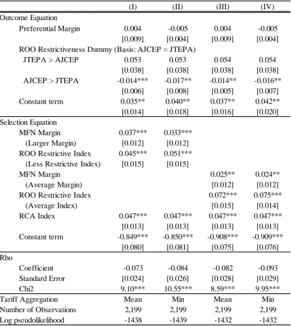
In the following, we report results for some kinds of robustness checks. In Table 6, we replace a continuous variable of ROO Difference with its dummy variable indicating which preferential scheme imposes the more restrictive ROOs. This replacement is because one possible source for the unexpected results in ROO Difference in Table 5 might be the way of scoring, i.e. adding the value “one” according to levels of ROO restrictiveness. In order to relax this restrictive and arbitral ordering, we introduce the binary variable on differences in ROO restrictiveness between AJCEP and JTEPA. The results in this new variable are more consistent with our expectation than those in Table 5. The dummy indicating the more restrictive ROOs in JTEPA has insignificant results, but the coefficients for the dummy indicating the more restrictive ROOs in AJCEP are estimated to be significantly negative. Namely, the products with the more restrictive ROOs in AJCEP than in JTEPA are less likely to be exported under the AJCEP scheme. The results in the other variables are qualitatively unchanged. Since the basis for the above new ROO dummy variables is the products having the common ROO restrictiveness between AJCEP and JTEPA, we can still interpret directly constant terms in this table as indicating the trade creation effect of diagonal cumulation, which is estimated to be around 4%.
=== Table 6 ===
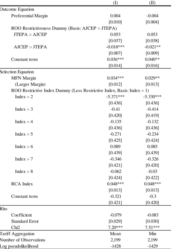
Due to a similar reason, in Table 7 we introduce dummy variables indicating scores of the ROO Restrictive Index into the selection equation rather than its continuous variable. Here we focus on the ROO Restrictive Index based on the less restrictive index because that based on the average index has so much variation in values. The results in those dummy variables are surprising. Under the basis of the
13
restrictiveness in CS/RVC or CS/RVC/TECH, only CS shows a significantly different restrictiveness. Namely, the criterion of Change in Subsection is the most restrictive ROOs in AJCEP and JTEPA. It is difficult to interpret this result well. We may say at least that ROOs in AJCEP and JTEPA are not determined in a similar way as the cases of FTAs in the United States and Europe. The results in the other variables are qualitatively unchanged. The estimates of constant terms in the outcome equation again show around 4% trade creation effect of the diagonal cumulation rule.
=== Table 7 ===
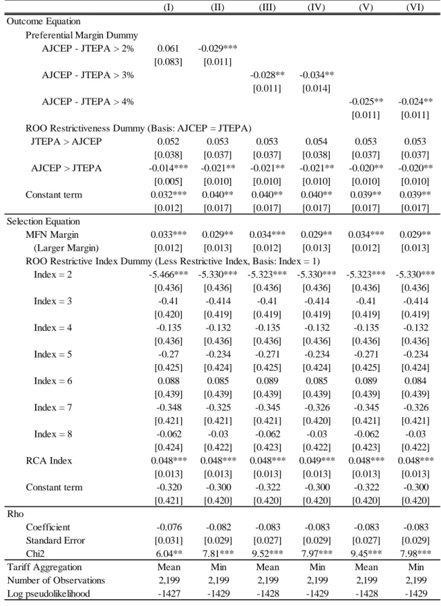
Lastly, we modify the preferential margin in the outcome equation. Specifically, we introduce a dummy variable indicating whether AJCEP rates are 2%, 3%, or 4% higher than JTEPA rates rather than a continuous variable of the preferential margin. Since products with lower rates in AJCEP than in JTEPA occupy only around 0.5% of all products even at the six-digit level (remember that Table 1 is at the nine-digit level), we do not introduce a dummy variable indicating whether or not AJCEP rates are lower than JTEPA rates. The products with 2% higher rates in AJCEP occupy around 5% of all products. Indeed, in our estimation sample, around 85% of products have equal tariff rates between AJCEP and JTEPA. The estimation results are reported in Table 8. Except for the case of column (I), all preferential margin dummy variables have significantly negative coefficients, indicating that products with much higher rates in AJCEP are less likely to be exported under AJCEP. It is interesting that the absolute magnitude of the coefficients is largest in the case of 3% difference. This result may indicate that the introduction of the diagonal cumulation rule is equivalent to having around 3% difference in preferential tariff rates. The results in the other variables are qualitatively unchanged. In particular, although the basis for the above new dummy variables is not exactly the products with no differences between AJCEP and JTEPA rates, the estimates of constant terms are quantitatively unchanged.
=== Table 8 ===
5. Concluding Remarks
In this paper, we empirically investigated the effect of diagonal cumulation on FTA utilization by exploring Thai exports to Japan under the JTEPA and AJCEP schemes. While JTEPA adopts bilateral cumulation, AJCEP does diagonal cumulation.
14
With these two FTA schemes, unlike previous studies, we can examine the effect of diagonal cumulation without relying on the variation in cumulation rules not only across country pairs but also across years. In short, our estimates do not suffer from biases from the effects of time-variant or country pair-specific elements. This is possible because we can compare trade in a country pair under FTA with diagonal cumulation with trade in the same pair under FTA without diagonal cumulation, for the identical product in the identical year. As a result, our estimates show around 4% trade creation effect of diagonal cumulation, which is much smaller than the estimates in the previous studies (around 15%). Thus, those in the previous studies may overestimate the trade creation effect of diagonal cumulation due to the inclusion of the effects of unobservable time-variant elements and country pair-specific elements.
15
Appendix. Score of ROOs Restrictiveness Index
ROO Type Score
CS/RVC 1 CS/RVC/TECH 1 CS 2 CH/RVC 3 CH/RVC/TECH 3 CH/TECH 3 CH 4 RVC 4 CH&RVC 5 CH&TECH 5 CC/RVC 6 CC 7 CC&TECH 8 WO 8
Notes: “CS”, “CH”, and “CC” are the ROO criteria of “Change in Subheading”, “Change in
Heading”, and “Change in Chapter”, respectively. “WO” indicates wholly-obtained criterion. “RVC” is the ROO criteria of the less than 40% real value-added content. “TECH” is the specific manufacturing or processing operations criterion.
Source: Author’s compilation based on the method proposed in Estevadeordal (2000) and
16
References
Augier, P., Gasiorek, M., and Tong, C.L., 2005, The Impact of Rules of Origin on Trade Flows, Economic Policy, 20(43): 567-624.
Bureau, J., Chakir, R., and Gallezot, J., 2007, The Utilisation of Trade Preferences for Developing Countries in the Agri-food Sector, Journal of Agricultural Economics,
58(2): 175-198.
Cadot, O. and de Melo, J., 2007, Why OECD Countries Should Reform Rules of Origin,
World Bank Research Observer, 23(1): 77-105.
Cadot, O., Carrere, C., De Melo, J., and Tumurchudur, B., 2006, Product-specific Rules of Origin in EU and US Preferential Trading Arrangements: An Assessment,
World Trade Review, 5(2): 199-224.
Demidova, S. and Krishna, K., 2008, Firm Heterogeneity and Firm Behavior with Conditional Policies, Economics Letters, 98(2): 122-128.
Estevadeordal, A., 2000, Negotiating Preferential Market Access: The case of the North American Free Trade Agreement, Journal of World Trade, 34: 141-200.
Estevadeordal, A. and Suominen, K., 2004, Rules of Origin in FTAs in Europe and in the Americas: Issues and Implications for the EU-Mercosur Inter-Regional Association Agreement, INTAL-ITD Working Paper 15.
Estevadeordal, A. and Suominen, K., 2008, What are the Effects of Rules of Origin on Trade?, In: Estevadeordal, A. and Suominen, K. (Eds.) Rules of Origin and
International Economic Integration, 161-219.
Francois, J., Hoekman, B., and Manchin, M., 2006, Preference Erosion and Multilateral Trade Liberalization, World Bank Economic Review, 20(2): 197-216.
Hakobyan, S., 2010, Accounting for Underutilization of Trade Preference Programs: U.S. Generalized System of Preferences, mimeo, University of Virginia.
Hansen, B., 2000, Sample Splitting and Threshold Estimation, Econometrica, 68(3), 575-604.
Hayakawa, K., 2011, Measuring Fixed Costs for Firms’ Use of a Free Trade Agreement: Threshold Regression Approach, Economics Letters, 113(3): 301-303.
Innwon, P. and Soonchan, P., 2009, Consolidation and Harmonization of Regional Trade Agreements (RTAs): A Path toward Global Free Trade, MPRA Paper No. 14217. Manchin, M., 2006, Preference Utilisation and Tariff Reduction in EU Imports from
17
Table 1. MFN Rates, AJCEP Preferential Rates, and JTEPA Preferential Rates Number of Tariff-line Share MFN vs. AJCEP 0 < MFN − AJCEP ≤ 3 958 23% 3 < MFN − AJCEP ≤ 5 1,527 37% 5 < MFN − AJCEP ≤ 10 1,420 34% 10 < MFN − AJCEP ≤ 20 234 6% MFN − AJCEP > 20 13 0.3% MFN vs. JTEPA 0 < MFN − JTEPA ≤ 3 711 17% 3 < MFN − JTEPA ≤ 5 1,539 37% 5 < MFN − JTEPA ≤ 10 1,625 39% 10 < MFN − JTEPA ≤ 20 255 6% MFN − JTEPA > 20 22 1% AJCEP vs. JTEPA AJCEP − JTEPA > 10 5 0.1% 5 < AJCEP − JTEPA ≤ 10 55 1% 3 < AJCEP − JTEPA ≤ 5 102 2% 1 < AJCEP − JTEPA ≤ 3 389 9% 0 < AJCEP − JTEPA ≤ 1 133 3% AJCEP − JTEPA = 0 3,462 83% -1 ≤ AJCEP − JTEPA < 0 6 0.1% AJCEP − JTEPA < -1 0 0%
Source: World Integrated Trade Solution Database Note: Tariff-line is defined at the 9-digit level.
18 Table 2. Rules of Origin: AJCEP and JTEPA
CC CC CC CH CH CH CH CH CH CS CS CS RVC WO ALL
/RVC &TECH /RVC /TECH /RVC &RVC &TECH /RVC /RVC
JTEPA /TECH /TECH
CC 411 90 6 17 524 CC/RVC 2 1 48 21 72 CC&TECH 266 1 267 CH 73 62 31 81 247 CH/RVC 13 181 2 196 CH/TECH 10 10 CH/RVC/TECH 345 345 CH&RVC 1 1 CH&TECH 43 183 226 CS 4 1 22 2 29 CS/RVC 18 9 27 CS/RVC/TECH 236 236 RVC 3 3 WO 1 15 16 ALL 490 15 399 69 923 0 0 1 264 2 11 0 24 1 2,199 AJCEP
Source: Legal texts of AJCEP and JTEPA Note: Tariff-line is defined at the 6-digit level.
19
Table 3. FTA Utilization Rates: AJCEP and JTEPA (US Dollar) Section
ALL AJCEP JTEPA AJCEP JTEPA
Live animals 552,768 96 524,625 0.0% 95%
Vegetable products 178,237 9 159,148 0.0% 89%
Food products 1,740,739 5,721 1,435,688 0.3% 82%
Beverage and tobacco 261,795 0 1,925 0% 1%
Mineral products 433,146 178 280,116 0.0% 65%
Chemical products 804,553 8,121 682,065 1.0% 85%
Plastics and rubber 49,641 53 27,228 0.1% 55%
Leather products 46,894 1,193 34,964 2.5% 75%
Wood products 580,143 4,334 458,124 0.7% 79%
Footwear 39,451 312 24,149 0.8% 61%
Non-metallic mineral products 131,060 23 106,148 0.0% 81%
Metal products 117,433 0 98,379 0% 84%
Machinery 431,964 22 391,916 0.0% 91%
Transport equipment 251,316 0 19,010 0% 8%
Precision machinery 0 0 0
Arms and ammunition 1,185 0 1 0% 0.1%
Miscellaneous manufac. 181,974 0 126,022 0% 69%
ALL 5,802,300 20,063 4,369,508 0.3% 75%
Exports Utilization
Source: Author compilation from official records of the certificates of origin available at the Bureau
20 Table 4. Baseline Results on Heckman Estimation
Variable Obs Mean Std. Dev. Min Max
Dep. Var. in Outcome Equation 790 0.025 0.256 0 4.8025
Preferential Margin (Mean) 790 0.366 1.057 -0.5 8.96
Preferential Margin (Min) 790 0.317 1.026 0 10.2
ROO Difference 790 0.149 1.103 -5 5
Dep. Var. in Selection Equation 2,199 0.359 0.480 0 1
MFN Margin (Larger Margin & Mean) 2,199 5.070 2.739 1 22.4
MFN Margin (Larger Margin & Min) 2,199 4.665 2.582 0.5 22.4
MFN Margin (Average Margin & Mean) 2,199 4.928 2.678 0.4333 21.85 MFN Margin (Average Margin & Min) 2,199 4.537 2.533 -0.95 21.85 ROO Restrictive Index (Less Restrictive Index) 2,199 5.268 2.050 1 8
ROO Restrictive Index (Average Index) 2,199 4.928 2.095 1 8
21 Table 5. Baseline Results on Heckman Estimation
(I) (II) (III) (IV)
Outcome Equation Preferential Margin 0.002 -0.006 0.002 -0.006 [0.010] [0.005] [0.010] [0.005] ROO Difference 0.016 0.017* 0.016 0.017* [0.010] [0.010] [0.010] [0.010] Constant term 0.041** 0.046** 0.043** 0.048** [0.017] [0.020] [0.018] [0.021] Selection Equation MFN Margin 0.037*** 0.033*** (Larger Margin) [0.012] [0.012] ROO Restrictive Index 0.045*** 0.051*** (Less Restrictive Index) [0.015] [0.015]
MFN Margin 0.025** 0.024**
(Average Margin) [0.012] [0.012]
ROO Restrictive Index 0.072*** 0.075***
(Average Index) [0.015] [0.014] RCA Index 0.047*** 0.047*** 0.047*** 0.047*** [0.013] [0.013] [0.013] [0.013] Constant term -0.850*** -0.850*** -0.908*** -0.909*** [0.080] [0.081] [0.075] [0.076] Rho Coefficient -0.074 -0.085 -0.081 -0.091 Standard Error [0.025] [0.027] [0.028] [0.029] Chi2 8.44*** 10.09*** 8.24*** 9.53***
Tariff Aggregation Mean Min Mean Min
Number of Observations 2,199 2,199 2,199 2,199
Log pseudolikelihood -1439 -1440 -1433 -1433
Notes: The dependent variables in outcome and selection equations are the ratio of exports under
AJCEP to those under JTEPA and the indicator variable on the use of the FTA preferential scheme, respectively. The model is estimated via the maximum likelihood estimation technique. The parentheses are robust standard errors. ***, **, and * show 1%, 5%, and 10% significance, respectively.
22
Table 6. Robustness Check: Comparing ROO Restrictiveness
(I) (II) (III) (IV)
Outcome Equation
Preferential Margin 0.004 -0.005 0.004 -0.005
[0.009] [0.004] [0.009] [0.004] ROO Restrictiveness Dummy (Basis: AJCEP = JTEPA)
JTEPA > AJCEP 0.053 0.053 0.054 0.054 [0.038] [0.038] [0.038] [0.038] AJCEP > JTEPA -0.014*** -0.017** -0.014** -0.016** [0.006] [0.008] [0.005] [0.007] Constant term 0.035** 0.040** 0.037** 0.042** [0.014] [0.018] [0.016] [0.020] Selection Equation MFN Margin 0.037*** 0.033*** (Larger Margin) [0.012] [0.012] ROO Restrictive Index 0.045*** 0.051*** (Less Restrictive Index) [0.015] [0.015]
MFN Margin 0.025** 0.024**
(Average Margin) [0.012] [0.012]
ROO Restrictive Index 0.072*** 0.075***
(Average Index) [0.015] [0.014] RCA Index 0.047*** 0.047*** 0.047*** 0.047*** [0.013] [0.013] [0.013] [0.013] Constant term -0.849*** -0.850*** -0.908*** -0.909*** [0.080] [0.081] [0.075] [0.076] Rho Coefficient -0.073 -0.084 -0.082 -0.093 Standard Error [0.024] [0.026] [0.028] [0.029] Chi2 9.10*** 10.55*** 8.59*** 9.95***
Tariff Aggregation Mean Min Mean Min
Number of Observations 2,199 2,199 2,199 2,199
Log pseudolikelihood -1438 -1439 -1432 -1432
23
Table 7. Robustness Check: Decomposing ROO Restrictiveness
(I) (II)
Outcome Equation
Preferential Margin 0.004 -0.004
[0.010] [0.004]
ROO Restrictiveness Dummy (Basis: AJCEP = JTEPA)
JTEPA > AJCEP 0.053 0.053 [0.037] [0.038] AJCEP > JTEPA -0.018*** -0.021** [0.007] [0.009] Constant term 0.036*** 0.040** [0.014] [0.016] Selection Equation MFN Margin 0.034*** 0.029** (Larger Margin) [0.012] [0.013]
ROO Restrictive Index Dummy (Less Restrictive Index, Basis: Index = 1)
Index = 2 -5.371*** -5.330*** [0.436] [0.436] Index = 3 -0.41 -0.414 [0.420] [0.419] Index = 4 -0.135 -0.132 [0.436] [0.436] Index = 5 -0.271 -0.234 [0.425] [0.424] Index = 6 0.089 0.085 [0.439] [0.439] Index = 7 -0.346 -0.326 [0.421] [0.420] Index = 8 -0.062 -0.03 [0.424] [0.422] RCA Index 0.048*** 0.048*** [0.013] [0.013] Constant term -0.321 -0.3 [0.421] [0.420] Rho Coefficient -0.079 -0.083 Standard Error [0.029] [0.030] Chi2 7.20*** 7.51***
Tariff Aggregation Mean Min
Number of Observations 2,199 2,199
Log pseudolikelihood -1428 -1429
Notes: See notes in Table 4. The scoring rule for the ROO Restrictive Index is available in the
24
Table 8. Robustness Check: Decomposing Preferential Margin
(I) (II) (III) (IV) (V) (VI) Outcome Equation
Preferential Margin Dummy
AJCEP - JTEPA > 2% 0.061 -0.029*** [0.083] [0.011] AJCEP - JTEPA > 3% -0.028** -0.034** [0.011] [0.014] AJCEP - JTEPA > 4% -0.025** -0.024** [0.011] [0.011] ROO Restrictiveness Dummy (Basis: AJCEP = JTEPA)
JTEPA > AJCEP 0.052 0.053 0.053 0.054 0.053 0.053 [0.038] [0.037] [0.037] [0.038] [0.037] [0.037] AJCEP > JTEPA -0.014*** -0.021** -0.021** -0.021** -0.020** -0.020** [0.005] [0.010] [0.010] [0.010] [0.010] [0.010] Constant term 0.032*** 0.040** 0.040** 0.040** 0.039** 0.039** [0.012] [0.017] [0.017] [0.017] [0.017] [0.017] Selection Equation MFN Margin 0.033*** 0.029** 0.034*** 0.029** 0.034*** 0.029** (Larger Margin) [0.012] [0.013] [0.012] [0.013] [0.012] [0.013] ROO Restrictive Index Dummy (Less Restrictive Index, Basis: Index = 1)
Index = 2 -5.466*** -5.330*** -5.323*** -5.330*** -5.323*** -5.330*** [0.436] [0.436] [0.436] [0.436] [0.436] [0.436] Index = 3 -0.41 -0.414 -0.41 -0.414 -0.41 -0.414 [0.420] [0.419] [0.419] [0.419] [0.419] [0.419] Index = 4 -0.135 -0.132 -0.135 -0.132 -0.135 -0.132 [0.436] [0.436] [0.436] [0.436] [0.436] [0.436] Index = 5 -0.27 -0.234 -0.271 -0.234 -0.271 -0.234 [0.425] [0.424] [0.425] [0.424] [0.425] [0.424] Index = 6 0.088 0.085 0.089 0.085 0.089 0.084 [0.439] [0.439] [0.439] [0.439] [0.439] [0.439] Index = 7 -0.348 -0.325 -0.345 -0.326 -0.345 -0.326 [0.421] [0.421] [0.421] [0.420] [0.421] [0.421] Index = 8 -0.062 -0.03 -0.062 -0.03 -0.062 -0.03 [0.424] [0.422] [0.423] [0.422] [0.423] [0.422] RCA Index 0.048*** 0.048*** 0.048*** 0.049*** 0.048*** 0.048*** [0.013] [0.013] [0.013] [0.013] [0.013] [0.013] Constant term -0.320 -0.300 -0.322 -0.300 -0.322 -0.300 [0.421] [0.420] [0.420] [0.420] [0.420] [0.420] Rho Coefficient -0.076 -0.082 -0.083 -0.083 -0.083 -0.083 Standard Error [0.031] [0.029] [0.027] [0.029] [0.027] [0.029] Chi2 6.04** 7.81*** 9.52*** 7.97*** 9.45*** 7.98***
Tariff Aggregation Mean Min Mean Min Mean Min
Number of Observations 2,199 2,199 2,199 2,199 2,199 2,199 Log pseudolikelihood -1427 -1429 -1428 -1429 -1428 -1429
Notes: See notes in Table 4. The scoring rule for the ROO Restrictive Index is available in the