A Continuum Dynamics on Vector Bundle (Geometric Mechanics)

A

Continuum Dynamics

on

Vector Bundle

理化学研究所 山岡英孝 (Hidetaka Yamaoka)1

Computational Cell Biomechanics Team,

VCAD System Research Program,

RIKEN

Abstract

The Cosserat theory for continua with microstructure can be geometrically

inter-preted as a continuum dynamics on vector bundle. In this talk, we begin with

ge-ometrical settings for the continua with microstructure and construct its dynamics

as continuum dynamics on vector bundle. As an example, we deal with a Cosserat

rod, which is considered as a one-dimensional continuum with microstructure. In

addition, we suggest thatwe can describelowermicrostructure ofthe elasticrods, by

extending the base manifold of the vector bundle to athree-dimensional continuum.

Such rodmodel well represents biomolecules involvingvarious interacting factors, so

that the model can be applied to analysis ofdeformation behavior ofbiomolecules.

We expect that our geometrical method would contribute to development of the

molecular biomechanics.

1

Introduction

We attempt to

construct

geometrical foundations and dynamical frameworks of

a

directed

medium based

on

the fiber bundle theory. The directed medium is

a

continuum with

microstructures that is described by a deformable vector, called

a

director. Studies

on

the

directed medium were actively pursued in the $1960s$, for example, by Ericksen [1], Toupin

[2], and Eringen and

_{\S uhubi}

[3] and in recent years, have been investigated from many

point of views such

as

elast-plasticity [4, 5], advanced materials [6], and biomechanics

[7, 8]. In contrast, since about the $1960s$, the elastic theory has been reconstructed using

differential geometry, for example, by Green and Rivilin [9], Noll [10], and Wang [11].

A modern text by Marsden and Hughes [12] helps us to consider geometrical settings of

elasticity (see also

an

early textbook [13]). In this study, we develop the dynamics of the

directed medium based

on

the fiber bundle theory in differential geometry.

In geometric continuum mechanics,

an

elastic body is viewed as

a

differentiable

mani-fold, while

a

directed medium is viewed

as a

vector bundle whose fiber denotes

a

collection

of the deformable directors. Hence, the mechanical behaviors of the directed medium

should be described

as

the continuum dynamics on a tangent bundle of

a

vector bundle.

Thus, we begin with a geometrical setting ofthe continuum dynamics on a vector bundle,

and derive

a

weak form and equations of motion for the directed medium. For future

applications,

we use

elasticity notations to provide

a

framework of continuum dynamics

on the vector bundle and present

some

figures for better understanding. Moreover,

we

apply

our

resultant equations to

a

Cosserat rod,

as

an

example, and find that the derived

equations of motion coincide with the balance laws of large deformable rods. It is simple

to prove such

a

coincidence if the equations of motion

are

restricted to the special Cosserat

rod with undeformed cross-section.

We

can use our

description to examine such macro-micro

interactive

mechanisms, if

we

have to consider only the geometrical structures of objects using the mechanisms,

i. e., the corresponding base manifolds and fiber spaces. Such geometrical considerations

help

us

to improve

our

understanding of the complicated mechanical behaviors ofvarious

structures associated with the macro-micro interactive mechanisms.

2

Geometry and

kinematics

In the geometric continuum mechanics,

an

elastic body is viewed

as

an

m-dimen-sional

Riemannian manifold $\mathcal{B}$, and deforms in

an

ambient space $S$,

an

n-dimen-sional Rieman-nian manifold $(m\leq n)[12]$

.

In contrast, when

we

_consider

a deformation

_of

_a

_continuum

with microstructure,

we

must

replace

these manifolds

with principal

fiber

bundles, de-noting by $\mathcal{P}$ and

2,

respectively,

over

the manifolds $\mathcal{B}$ and $S$. The

microstructure

is often expressed by a r-dimensional vector $(r\leq n)$, called director. In this case, the space

consisting of the directors, 7, is exactly the fiber of the bundle $\mathcal{P}arrow \mathcal{B}$, and then $\mathcal{P}$

can

be considered

as

the real vector bundle $g\simeq \mathcal{B}\cross 7$

.

A configuration of the continuum with

microstructure

is given by

a

smooth embedding

$\Phi$ : $\mathcal{P}arrow 2$, then the configuration space is

a

space of all embeddings,

$=$

_{

$\Phi$ : $\mathcal{P}arrow 2$, smooth

embedding}.

(2.1)

Indeed, for

an

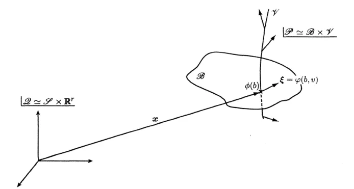
arbitrary point$p=(b, v)\in \mathcal{P}\simeq \mathcal{B}\cross\gamma/(b\in \mathcal{B}$ and _{$v\in\gamma)$},

we can

define

the embedding $\Phi$ through embedding of the

base

manifold $\phi$ : $\mathcal{B}arrow S$ and projection

onto the fiber $\varphi$ : $\mathcal{B}\cross 7arrow \mathbb{R}^{r}$;

$\Phi(p)=(\phi(b), \varphi(b, v))$. (2.2)

It is easy to verify that this map is the embedding. We note here that the ambient bundle

J2 is the vector bundle $9arrow S$ _{with fiber} $\mathbb{R}^{r}$, i. e., _{$9arrow S\cross \mathbb{R}^{r}$}

,

as

shown in Fig. 1.

For sake of simplicity, we take the ambient space

as

the n-dimensional Euclidean

space; $S\simeq \mathbb{R}^{n}$, and

we

embed the fiber space $\mathbb{R}^{r}$ into the

same

Euclidean space $\mathbb{R}^{n}$.

Then

we

denote position vectors of points in the reference body $\mathcal{B}_{0}$ and current body

$\mathcal{B}$ by

$X=\phi_{0}(b_{0})(b_{0}\in \mathcal{B}_{0})$ and $x=\phi(b)(b\in \mathcal{B})$, respectively. Also,

we

denote

reference and current directors associated with their points by $\Xi=\varphi_{0}(b_{0}, v_{0})(v_{0}\in 7_{0}’)$

and $\xi=\varphi(b, v)(v\in Y)$,

as

shown Fig. 1. Accordingly, three deformation _{gradient tensors}

can

be defined

as

$F= \frac{\partial x}{\partial X}$, $\mathfrak{F}=\frac{\partial\xi}{\partial X}$, $\mathcal{F}=\frac{\partial\xi}{\partial_{-}^{-}-}$,

(2.3)

Figure 1: Illustration ofthe continuum with microstructure, $\mathcal{P}\simeq \mathcal{B}\cross 7$, embedded into

the ambient bundle, $\ovalbox{\tt\small REJECT}\simeq S\cross \mathbb{R}^{r}$, and its local coordinates in

2.

Since the trivialization of bundle 2 is expressed as

$9\simeq S\cross \mathbb{R}^{r}$, (2.4)

the flat connection is defined

on

the bundle

2.

Accordingly, the tangent bundle

T.2

is

decomposed into the tangent bundles $TS$ _and $T\mathbb{R}^{r}$;

$T2\simeq TS\oplus T\mathbb{R}^{r}$

.

(2.5)

Also, the cotangent bundle $T^{*}9$ is decomposed by the flat connection,

so

that one-form

$dq\in T_{q}^{*}2$ is put in the form

$dq=dx+d\xi$, (2.6)

and expressed, in terms of the reference coordinates $q_{0}=(X, \Xi)$,

as

$dq=(F+\mathfrak{F})dX+\mathcal{F}d\Xi$

.

(2.7)

From Eq. (2.7), the quadratic form $dq^{2}$ is calculated

as

$dq^{2}=dX^{T}(F+\mathfrak{F})^{T}(F+\mathfrak{F})dX$

$+dX^{T}(F+\mathfrak{F})^{T}\mathcal{F}d\Xi+d\Xi^{T}\mathcal{F}^{T}(F+\mathfrak{F})dX$

$+d\Xi^{T}\mathcal{F}^{T}\mathcal{F}d\Xi$, (2.8)

where $T$ denotes the transposition of tensors. Here,

we

set

$C=(F+\mathfrak{F})^{T}(F+\mathfrak{F})$, (2.9a)

$C=\mathcal{F}^{T}\mathcal{F}$, (2.9b) $C=\mathcal{F}^{T}(F+\mathfrak{F})$, (2.9c)

called

macro

deformation, micro deformation, and (macro-micro) mixture deformation,

respectively. The reference deformations put in the form

$C_{0}=(I+\mathfrak{F}_{0})^{T}(I+\mathfrak{F}_{0})$, (2.10a)

$C_{0}=I$, (2.10b)

$C_{0}=I^{T}(I+\mathfrak{F}_{0})$, (2.10c)

where $I$ is n-th order identity tensor, and where $\mathfrak{F}_{0}=\partial\Xi/\partial X$,

as

well. Thus,

we

have

the difference of the current and reference quadratic forms,

$dq^{2}-dq_{0}^{2}=dX^{T}(C-C_{0})dX$

$+dX^{T}(C-C_{0})^{T}d\Xi+d\Xi^{T}(C-C_{0})dX$

$+d\Xi^{T}(C-C_{0})d\Xi$, (2.11)

so that we define the strains as

$E= \frac{1}{2}(C-C_{0})$, (2.12a)

$\mathcal{E}=\frac{1}{2}(C-C_{0})$, (2.12b) $\not\subset=\frac{1}{2}(C-C_{0})$. (2.12c)

Then we call them macro strain, micro strain, and (macro-micro) mixture strain,

re-spectively. Here, we comment

on

the terminologies used by Eringen’s textbook for the

microcontinuum [14]. In the textbook, our mixture deformation $C$ is decomposed into

$\mathcal{F}^{T}F$ and $\mathcal{F}^{T}\mathfrak{F}$, called the Cosserats deformation tensor, when the director is deformed

rigidly, “micropolar continua” according to the textbook, and the wryness tensor,

respec-tively. Additionally, the micro deformation tensor is defined in the

same

manner, while

the

macro

deformation tensor is linearized to $F^{T}F$_.

3

Dynamics

Now, we consider a Lagrangian$\mathcal{L}=\mathcal{T}-\mathcal{W}$, where $\mathcal{T}$ is the kinetic energy,

defined through

a metric on , and $\mathcal{W}$ is a potential function on . Then the dynamics of the continuum

with microstructure is described

on

the tangent bundle $T$ of the configuration space ,

that is, the Lagrangian $\mathcal{L}$ is defined

as

a function of the tangent bundle $T$ to $\mathbb{R}$,

$\mathcal{L}(\Phi,\dot{\Phi})=\mathcal{T}(\Phi,\dot{\Phi})-\mathcal{W}(\Phi)$. (3.1)

Usually, the strain energy $\mathcal{W}(\Phi)$ is expressed

as

a functional of $\psi$, which is difined as a

function of the deformation gradient tensors $F_{:}\mathfrak{F}$, and $\mathcal{F}$:

$\mathcal{W}(\Phi)=\int_{p}\psi(F, \mathfrak{F}, \mathcal{F})dV$. (3.2)

We also denote the Lagrangian and kinetic enegy densities by $\mathcal{L}$ and ,9, respectively,

i.e., $\mathcal{L}=\int \mathcal{L}dV$ and $\mathcal{T}=\int\ovalbox{\tt\small REJECT} dV$, and, for simplicity, we consider those densities as

functions of the local coordinates $(x, \xi,\dot{x},\dot{\xi})$ on the tangent bundle $T\ovalbox{\tt\small REJECT}$. In this case, the

Hamilton’s principle for any time interval $[t_{0}, t_{1}]$ is expressed

as

follows:

$\int_{t_{0}}^{t_{1}}\int_{\Phi(\mathcal{P})}(\frac{\partial \mathcal{L}}{\partial x}$

.

$\delta x+\frac{\partial \mathcal{L}}{\partial\dot{x}}$ . $\delta\dot{x}+\frac{\partial \mathcal{L}}{\partial\xi}$ . $\delta\xi+\frac{\partial \mathcal{L}}{\partial\dot{\xi}}$ . $\delta\dot{\xi}$

$+ \frac{\partial \mathcal{L}}{\partial F}$ : $\delta F+\frac{\partial \mathcal{L}}{\partial \mathfrak{F}}$ : $\delta \mathfrak{F}+\frac{\partial \mathcal{L}}{\partial \mathcal{F}}$ : _{$\delta \mathcal{F})\Phi(dV)dt=0$}, (3.3)

where

we

have denoted, by. and :, the inner product of vectors and double contraction

of tensors, respectively,

or

equivalently the simple-dot and double-dot products in the

dyadics. Then, by performing partial integration and using the divergence theorem,

we

obtain the weak form for the continuum with microstructure,

$\int_{t_{0}}^{t_{1}}\int_{\Phi(9)}[(\frac{\partial}{\partial t}(\frac{\partial ff}{\partial\dot{x}})-\frac{\partial F}{\partial x}-\frac{\partial}{\partial X}\cdot(\frac{\partial\Psi}{\partial F}))\cdot\delta x$

$+( \frac{\partial}{\partial t}(\frac{\partial F}{\partial\dot{\xi}})-\frac{\partial\ovalbox{\tt\small REJECT}}{\partial\xi}-\frac{\partial}{\partial X}\cdot(\frac{\partial\psi}{\partial \mathfrak{F}})-\frac{\partial}{\partial_{-}^{-}-}\cdot(\frac{\partial\psi}{\partial \mathcal{F}}))\cdot\delta\xi]\Phi(dV)dt$

$+ \int_{t_{0}}^{t_{1}}\int_{\Phi(\partial 9)}[N\cdot\frac{\partial\Psi}{\partial F}\cdot\delta x+N\cdot(\frac{\partial\psi}{\partial \mathfrak{F}}+\frac{\partial\psi}{\partial \mathcal{F}})\cdot\delta\xi]\Phi(dA)dt=0$, (3.4)

where $\partial \mathcal{P}$ denotes the boundary of the material bundle $\mathcal{P}$, and $N$ and $dA$

are

the unit

normal to $\partial \mathcal{P}$ and the area form of $\partial \mathcal{P}$, respectively.

Finally, we assume that the Lagrangian density $\mathcal{L}=\ovalbox{\tt\small REJECT}-\psi$ has a compact support

and that the variations

are

fixed at the end points, $\delta x=\delta\xi=0(t=t_{0}, t_{1})$. Then

we

have equations of motion for the continuum with microstructure

$\frac{\partial}{\partial t}(\frac{\partial F}{\partial\dot{x}})=\frac{\partial ff}{\partial x}+\frac{\partial}{\partial X}\cdot(\frac{\partial\Psi}{\partial F})$ , (3.5a)

$\frac{\partial}{\partial t}(\frac{\partial ff}{\partial\dot{\xi}})=\frac{\partial ff}{\partial\xi}+\frac{\partial}{\partial X}\cdot(\frac{\partial\Psi}{\partial \mathfrak{F}})+\frac{\partial}{\partial_{-}^{-}-}\cdot(\frac{\partial\Psi}{\partial \mathcal{F}})$. (3.5b)

By introducing the generalized Piola-Kirchhoff stress tensors,

$P= \frac{\partial\psi}{\partial F}$, $\mathfrak{P}=\frac{\partial\Psi}{\partial \mathfrak{F}}$, $\mathcal{P}=\frac{\partial\psi}{\partial \mathcal{F}}$, (3.6)

we obtain the equations of motion, in terms of the generalized stress tensors,

$\frac{\partial}{\partial t}(\frac{\partial g}{\partial\dot{x}})=\frac{\partial ff}{\partial x}+P\cdot(\frac{\partial}{\partial X})$ , (3.7a)

$\frac{\partial}{\partial t,}(\frac{\partial ff}{\partial\dot{\xi}})=\frac{\partial F}{\partial\xi}+\mathfrak{P}\cdot(\frac{\partial}{\partial X})+\mathcal{P}\cdot(\frac{\partial}{\partial_{-}^{--}})$. (3.7b)

4

An

example:

Cosserat

rods

As

an

example,

we

consider a Cossrat rod laid in the _{three-dimensional Euclidean space}

$\mathbb{R}^{3}(n=3)$. In this case, the bundle $\mathcal{P}$ is the Cosserat rod,

a one-dimensional continuum

$\mathcal{B}$ expresses the center axis of

rod, and the director attached to each point of $\mathcal{B}$ is the

three-dimensional

vector to describe points in the cross-section at each point

on

the axis

$(m=1, r=3)$. Then, it is enough that the vector bundle $e2$ is taken

as

$\mathbb{R}^{3}\cross \mathbb{R}^{3}$.

We parameterize a position vector $r(s, t)$ of an arbitrary _point

on

$\phi(\mathcal{B})$ by the

arc-length parameter $s$ and the time parameter $t$. We define

a

right-handed orthonormal

basis, $\{d_{1}(s, t), d_{2}(s, t), d_{3}(s, t)\}$, along $\phi(\mathcal{B})$ at $s$ with $d_{1}=\partial r/\partial s$, and introduce the

curvature vector $\kappa(s, t)$ in the current body through

$\frac{\partial d_{k}}{\partial s}=\kappa\cross d_{k}$.

(4.1)

The component $\kappa^{1}=\langle d_{1},$$\kappa\}$ of $\kappa$ gives the torsion of _{$\phi(\mathcal{B})$} in the current configuration;

the two components, $\kappa^{\alpha}=\langle d_{\alpha},$ $\kappa\rangle,$ $\alpha=2,3$,

are

components of the

current curvature of

$\phi(\mathcal{B})$ and

are

related to the geometric curvature $\tilde{\kappa}$

of the current axial

curve

through the

formula

$(\tilde{\kappa})^{2}=(\kappa^{2})^{2}+(\kappa^{3})^{2}$. Then the

Cosserat

rod is provided

as

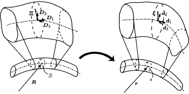
$x(s, t)=r(s, t)$, $\xi(s, t)=\xi^{k}d_{k}(s, t)$. _(4.2)

It is illustrated

as

Fig. 2. We

use

curvilinear coordinates with respect to $\{d_{k}\}$. Throughout

this article, _{the summation convention is used for repeated indices, with}

_Latin

_indices

taking the values

{1,

2,

_3}

and Greek indices taking the values

_{2,

_3}.

Figure 2: Illustration of the reference and current configurations of the Cosserat rod.

Additionally,

we

denote quantities _{for reference body by the capital letters of the}

corresponding

ones

for current body, that is, $R(S, 0)$ _{is the position vector of}

_an

ar-bitrary point

on

$\phi_{0}(\mathcal{B}_{0})$ by the arc-length parameter _$S$

$\{D_{1}(S,$ $0),$$D_{2}(S, 0),$ $D_{3}(S, 0)\}$ is aright-handed orthonormal basis along $\phi_{0}(\mathcal{B}_{0})$ at $S$ such

that $D_{1}=\partial R/\partial S$. Then, the reference curvature vector $\mathcal{K}_{0}(S, 0)$ is similarly defined by

$\frac{\partial D_{k}}{\partial S}=\mathcal{K}_{0}\cross D_{k}$. (4.3)

The component $\mathcal{K}_{0}^{1}=\langle D_{1},$ $\mathcal{K}_{0}\}$ of $\mathcal{K}_{0}$ gives the torsion of $\phi_{0}(\mathcal{B}_{0})$ in the reference

config-uration; the two components, $\mathcal{K}_{0}^{\alpha}=\langle D_{\alpha},$ $\mathcal{K}_{0}\rangle,$ $\alpha=2,3$, are components of the reference

curvature of $\phi_{0}(\mathcal{B}_{0})$ and

are

related to the geometric curvature

$\tilde{\mathcal{K}}_{0}$ of the reference axial

curve

through the formula $(\tilde{\mathcal{K}}_{0})^{2}=(\mathcal{K}_{0}^{2})^{2}+(\mathcal{K}_{0}^{3})^{2}$. Thus, the reference configuration is

provide

as

$X(S, 0)=R(S, 0)$, $\Xi(S, 0)=\Xi^{\alpha}D_{\alpha}(S, 0)$. (4.4)

It is shown

as

Fig. 2. Here,

we

consider that the reference configuration is unstressed

state, and then the cross-sections of the reference filament is

as

sumed to be normal to its

axial

curve.

If the cross-sections of the current filament remain normal to the current axial

curve,

we

may constrain $\xi^{1}=0$. When we suppose the special Cosserat rod, in which it

is assumed that the cross-sections of the current filament remain plane, undeformed, and

normal to the current axial curve,

we

have to append the constraints $\xi^{1}=0$ and $\xi^{\alpha}=\Xi^{\alpha}$.

Further, the extension $\epsilon(s, t)$ of the axial

curve

can

be defined through

$\frac{\partial s}{\partial S}=(1+\epsilon)$. (4.5)

Using the above the deference relation, we obtain the deformation gradients

$F=(1+\epsilon)d_{1}\otimes D^{1}$, (4.6a)

$\mathfrak{F}=(1+\epsilon)(\frac{\partial\xi^{k}}{\partial s}+\xi^{k}R(\kappa))d_{k}\otimes D^{1}$ , (4.6b)

$\mathcal{F}=\frac{\partial\xi^{k}}{\partial_{-}^{-\alpha}-}d_{k}\otimes D^{\alpha}$, (4.6c)

where $R(a)$ is the skew symmetric tensor associated with

a

polar vector $a$. Then the

current and reference deformations

are

calculated as, respectively,

$C=(1+ \epsilon)^{2}\Vert\frac{\partial}{\partial s}(r+\xi)\Vert^{2}D^{1}\otimes D^{1}$, (4.7a)

$\not\subset=\langle\frac{\partial\xi}{\partial_{-}^{-\alpha}-},$ $(1+ \epsilon)\frac{\partial}{\partial s}(r+\xi)\rangle D^{\alpha}\otimes D^{1}$ , (4.7b) $C= \langle\frac{\partial\xi}{\partial_{-}^{-\alpha}-},$ $\frac{\partial\xi}{\partial_{-}^{-\beta}-}\}D^{\alpha}\otimes D^{\beta}$, (4.7c)

and

$C_{0}= \Vert\frac{\partial}{\partial S}(R+\Xi)\Vert^{2}D^{1}\otimes D^{1}$ , (4.8a)

Co

$=\langle D_{\alpha},$ $\frac{\partial}{\partial S}(R+\Xi)\}D^{\alpha}\otimes D^{1}=\epsilon_{1\alpha\beta}\mathcal{K}_{0}^{1}\Xi^{\alpha}D^{\beta}\otimes D^{1}$ , (4.8b) $C_{0}=\delta_{\alpha\beta}D^{\alpha}\otimes D^{\beta}$, (4.8c)

where $\epsilon_{klm}$ is the Edinton’s epsilon, and $\Vert\cdot\Vert$ denotes the standard inner product on the

Euclidean spaces. Thus, we obtain the strains as follows:

$E= \frac{1}{2}[(1+\epsilon)^{2}\Vert d_{1}+\xi^{\alpha}R(\kappa)d_{\alpha}\Vert^{2}-\Vert D_{1}+\Xi^{\alpha}R(\mathcal{K}_{0})D_{\alpha}\Vert^{2}]D^{1}\otimes D^{1}$ , (4.9a)

$\not\subset=\frac{1}{2}[\langle\frac{\partial\xi}{\partial_{-}^{-\alpha}-},$$(1+ \epsilon)\frac{\partial}{\partial s}(r+\xi)\rangle-\langle D_{\alpha},$ $\frac{\partial}{\partial S}(R+\Xi)\rangle]D^{\beta}\otimes D^{1}$, (4.9b)

$\mathcal{E}=\frac{1}{2}[\langle\frac{\partial\xi}{\partial_{-}^{-\alpha}-},$$\frac{\partial\xi}{\partial_{-}^{-\beta}-}\}-\delta_{\alpha\beta}]D^{\alpha}\otimes D^{\beta}$. (4.9c)

Because of using the moving frame, we must rewrite the variational formulation. To

this end, we begin with defining the variation $\delta k$, associated with the orthonomal basis,

through

$\delta d_{k}=\delta k\cross d_{k}$, (4.10)

so

that the variation of the director $\xi$ is expressed

as

$\delta\xi=\delta k\cross\xi$, (4.11)

and the variations of the deformation gradients $F,$ $\mathfrak{F}$, and $\mathcal{F}$ become

$\delta F=\frac{\partial}{\partial R}(\delta r)+R(\delta k)F$, (4.12a)

$\delta \mathfrak{F}=\frac{\partial}{\partial R}(\delta\xi)+R(\delta k)\mathfrak{F}$, (4.12b) $\delta \mathcal{F}=\frac{\partial}{\partial_{-}^{-}-}(\delta\xi)+R(\delta k)\mathcal{F}$. (4.12c)

Then the weak form is rewretten

as

$\int_{t_{0}}^{t_{1}}\int_{\Phi(9)}[(\frac{\partial}{\partial t}(\frac{\partial F}{\partial\dot{r}})-\frac{\partial ff}{\partial r}-\frac{\partial}{\partial R}\cdot(\frac{\partial\psi}{\partial F}))\cdot\delta r$

$-( \frac{\partial\psi}{\partial F}$ : $R( \delta k)F+\frac{\partial\Psi}{\partial \mathfrak{F}}$ : $R( \delta k)\mathfrak{F}+\frac{\partial\Psi}{\partial \mathcal{F}}$ : $R(\delta k)\mathcal{F})$

$+( \xi\cross(\frac{\partial}{\partial t}(\frac{\partial ff}{\partial\dot{\xi}})-\frac{\partial ff}{\partial\xi}-\frac{\partial}{\partial R}\cdot(\frac{\partial\Psi}{\partial \mathfrak{F}})-\frac{\partial}{\partial_{-}^{-}-}\cdot(\frac{\partial\Psi}{\partial \mathcal{F}})))\cdot\delta k]\Phi(dV)dt$

$+ \int_{t_{0}}^{t_{1}}\int_{\Phi(\partial p)}[N\cdot\frac{\partial\psi}{\partial F}\cdot\delta r+\xi\cross(N\cdot(\frac{\partial\psi}{\partial \mathfrak{F}}+\frac{\partial\ovalbox{\tt\small REJECT}’}{\partial \mathcal{F}}))\cdot\delta k]\Phi(dA)dt=0$. (4.13)

Hence, under the fixed end points conditons, $\delta r=\delta k=0$, the equations of motion for

the Cosserat rod is derived

as

$\frac{\partial}{\partial t}(\frac{\partial F}{\partial\dot{r}})=\frac{\partial\ovalbox{\tt\small REJECT}}{\partial r}+\frac{\partial}{\partial R}\cdot(\frac{\partial\psi}{\partial F})$ , (4.14a)

$\xi\cross\frac{\partial}{\partial t}(\frac{\partial F}{\partial\dot{\xi}})=\xi\cross(\frac{\partial\ovalbox{\tt\small REJECT}}{\partial\xi}+\frac{\partial}{\partial R}\cdot(\frac{\partial\Psi}{\partial \mathfrak{F}}I+\frac{\partial}{\partial_{-}^{-}-}\cdot(\frac{\partial\psi}{\partial \mathcal{F}}))$

where $\cross$

denotes the cross-dot product in the dyadics, and it is defined

as

$(a_{1}\otimes a_{2})^{\cross}(a_{3}\otimes a_{4})=(a_{1}\cross a_{3})(a_{2}\cdot a_{4})$, (4.15)

for any vectors $a_{i}\in \mathbb{R}^{3}$.

In terms of the local coordinates, the kinetic enegy density is expressed

as

$eZ(r, \xi,\dot{r},\dot{\xi})=\frac{1}{2}\rho(r)(\Vert\dot{r}\Vert^{2}+\Vert\dot{\xi}\Vert^{2})$ , (4.16)

where $\rho(r)$ is

a

mass

density of the body at $r$ in the current configuration $\phi(\mathcal{B})$. Thus,

we obtain the equations of motion for the special Cosserat rods expressed in terms of the

generalized stress tensors,

$\frac{\partial}{\partial t}(\rho\dot{r})=\frac{1}{2}\frac{\partial\rho}{\partial r}\Vert\dot{r}\Vert^{2}+\frac{\partial}{\partial S}(P\cdot D^{1})$ , (4.17a)

$\xi\cross\frac{\partial}{\partial t}(\rho\dot{\xi})=\xi\cross(\frac{\partial}{\partial S}(\mathfrak{P}\cdot D^{1}+\mathcal{P}\cdot\Xi^{\alpha}R(\mathcal{K}_{0})^{T}D^{\alpha})+\frac{\partial}{\partial_{-}^{-\alpha}-}(\mathcal{P}\cdot D^{\alpha}))$

$+ \frac{\partial r}{\partial S}\cross(P\cdot D^{1})+\frac{\partial\xi}{\partial S}\cross(\mathfrak{P}\cdot D^{1}+\mathcal{P}\cdot D^{\alpha})+\frac{\partial\xi}{\partial_{-}^{-\alpha}-}\cross(\mathcal{P}\cdot D^{\alpha})$.

(4.17b)

By these expressions, it is well to reconstruct the balance laws for the Cosserat rod.

At the last in this section,

we

reduce the above equations to those for the special

Cosserat rod, that is, we impose the constraints $\xi^{1}=0$ and $\xi^{\alpha}=\Xi^{\alpha}$. In this case, the

micro deformation gradient becomes

$\mathcal{F}=\delta_{\beta}^{\alpha}d_{\alpha}\otimes D^{\beta}$, (4.18)

so

that the generalized micro stress tensor vanishes; $\mathcal{P}=0$, because of the assumption

about the undeformation of the cross-sections. Indeed, the micro strain vanishes, i. e.,

$\mathcal{E}=0$. Here, we note that the linearlized macro and mixture strains become

$E_{1inear}=\epsilon D^{1}\otimes D^{1}$, (4.19a) $C_{linear}=\frac{1}{2}\epsilon_{1\alpha\beta}(\kappa^{1}-\mathcal{K}_{0}^{1})\Xi^{\alpha}D^{\beta}\otimes D^{1}$. (4.19b)

Thenwe obtain the well-known equationsofmotion for the special Cosserat rods expressed

in terms of the generalized stress tensors,

$\frac{\partial}{\partial t}(\rho\dot{r})=\frac{1}{2}\frac{\partial\rho}{\partial r}\Vert\dot{r}\Vert^{2}+\frac{\partial}{\partial S}(P\cdot D^{1})$ , (4.20a)

$\xi\cross\frac{\partial}{\partial t}(\rho\dot{\xi})=\frac{\partial}{\partial S}(\xi\cross(\mathfrak{P}\cdot D^{1}))+\frac{\partial r}{\partial S}\cross(P\cdot D^{1})$ . (4.20b)

We comment that $P\cdot D^{1}$ and _{$\xi\cross(\mathfrak{P}\cdot D^{1})$} is exactly the stress and couple-stress along

5

Summary

In this study,

we

developed

formulations

for continuum dynamics

on a

tangent bundle of

a vector bundle that accurately _{describes the mechanical behavior of a directed medium.}

Indeed, the dynamics _{of the one-dimensional continuum with a director are well expressed}

as one

of the Cosserat rod, in which the cross-sectional structure is considered as the

microstructure

oftherod. For futuredevelopments, it is important to examinegeometrical

structures

of various continua with

_{microstructures.}

_{Especially, in the}

_case

_where

_we

consider

a

classification of microcontinua, it is necessary to _{investigate group actions}

on

the bodies and

microstructures.

For example, _{the group structures correspond to}

Eringen’s classification, i._{e., micromorphic, microstretch, and micropolar continua [14].}

Moreover,

we

can

extend the Cosserat rod to a model describing smaller

microstruc-ture of the elastic rod. Then the expressions for the smaller

_{microstructure}

_{to analyze}

deformation behavior of filaments _{including biopolymers. When a biopolymer expresses}

_a

certain function within a living organism, its conformation is an important factor that

de-termes the function. Therefore,

we

believe to obtain

a new

knowledge of the

interactions

between the dynamical situations and the biological

circumstances

of _{biopolymers, which}

have been _{investigated recently by considering the}

_deformation

_{behavior of biopolymers}

together with their

_{microstructures.}

References

[1] J. L. Ericksen,

_{“Conservation}

_{laws for liquid crystals,” Trans. Soc. Rheol., 5,}

_23-34

(1961).

[2] R. A. Toupin, _{“Theories of elasticity with couple-stress,” Arch. Ration. Mech. Anal.,}

17,

85-112

(1964).

[3] A. C. Eringen and E. S.

\S uhubi,

“Nonlinear theory of simple micro-elastic solids-I,”

Int. J. Eng. Sci., 2,

189-203

(1964).

[4] _{A. Riahi and J. H. Curran, Fu113D finite element}

_{Cosserat formulation}

_with

appli-cation in layered structures,” _{Appl. Math. Model., 33,}

_3450-3464

_(2009).

[5] S. Forest and R. Sievert, _{“Elastoviscoplastic constitutive}

_frameworks

_{for generalized}

continua,” Acta Mechanica, 160, 71-111 (2003).

[6] D. A. Burton _{and T. Gould, “Dynamical model of Cosserat nanotubes,” J. Phys.,}

62,

23-33

(2007).

[7] J. _{Rosenberg and R. Cirmrman,}

_{”Microcontinuum}

_{approach in}

_{biomechanical}

mod-eling,” Math. Comput. Simul., 61,

_249-260

(2003).

[8] K. A. Hohhman, R. S. Manning and J. H. Maddocks, _{“Link, twist, enegy and the}

stability of DNA minicircles,” Biopolymers, 70,

145-157

(2003).

[9] A. E. Green and R. S. Rivilin, “The mechanics ofnon-linear materials with memory,”

[10] W. Noll, “A mathematical theory of the mechanical behavior of continuous media,”

Arch. Ration. Mech. Anal., 2, 197-226 (1958).

[11] C.-C. Wang, “On the geometric structures of simple bodies,

a

mathematical founda-tion for the theory of continuous distributions of dislocations,” Arch. Ration. Mech.

Anal., 27, 33-94 (1967).

[12] J. E. Marsden and T. J.R. Hughes, Mathematical

_{foundations of}

elasticity,

Prentice-Hall, New York, 1983 (reprinted by Dover, New York, 1994).

[13] C.-C. Wang and C. Thruesdell, introduction to rational elasticity, Noordhoff

Interna-tional Publishing, Leyden, 1973.

[14] A. C. Eringen, Microcontinuum Field Theories: Foundations and Solids,