On the complete description of the Stokes geometry for the first Painleve hierarchy (Microlocal Analysis and Asymptotic Analysis)

On the

complete description

of

the

Stokes

geometry

for

the first

Painlev\’e

hierarchy

1

京都大学数理解析研究所 河合隆裕 (KAWAI, Takahiro)

RIMS, Kyoto University

京都大学理学研究科 小池達也 (KOIKE, Tatsuya)

Department of Mathematics, Kyoto University

京都大学数理解析研究所 西川享宏2 (NISHIKAWA, Yukihiro)

RIMS, Kyoto University

京都大学数理解析研究所 竹井義次 (TAKEI, Yoshitsugu)

RIMS, Kyoto University

We dedicate this paper to

Professor

Louis Boutet de Monvel

with

our

sincerest congratulations

on

his being awarded Prix deVEtat (Academie des

Science).

One

_of

the central issues

_of

this article is the introduction

_of

the notion

_of

virtual

tu rning points

_for

higher order Painlevi equations, and trvo

_of

the authors (Kawai

and $Takei)_{f}$ together with T. Aoki, fondly remember the stimula tlng and

comfort-able

_conference

(Algebraic analysis

_of

singular perturbations, 1991), which

Profes-sor Boutet de Monvel, together with

_Professor

M. Sato, organized, and where the

notion

_of

a

$v\dot{z}\hslash ual$ turning point

for

linear ordinary

differential

equations

was

first

made public (underthe modest

name

‘la

new

turning point”). The notion

_of

virtual

turning points is

one

_of

the most important gifts to the exact $WKB$ analysis

from

microlocal andysis, and hence

we

believe this article to be most appropriate to

ded-icate to

_Professor

Boutet de $Monvel_{\mathit{3}}$ who has made substantial contributions to the

development

_of

microlocal analysis and asymptotic analysis.

1

Introduction

As

was

first discovered numerically by Nishikawa [Nl, N2], Stokes

curves

of higher

order Painlev6 equations

cross

in general and

some

degeneracy ofStokes geometry

of the underlying Lax pair is often observed along

a

curved ray emanating from

such

a

crossing point of Stokes curves (”Nishikawaphenomenon ). To analyze this

intriguing phenomenon

we

investigated in [KKNT] several properties of the curved

this paperis in final form andnoversion of it will be submitted for publication elsewhere.

Current address: Government & Public Corporation Information Systems Division, Hitachi

ray, which

we

named

a

“new Stokes

curves

, bymaking full

use

of the underlyingLax

pair. The analysisdone in [KKNT] tells

us

that introduction of

new

Stokes

curves

is

inevitable to obtain a complete description ofthe global Stokes geometry of higher

order Painlev6 equations. In this report, using the results of [KKNT],

we

discuss

how to obtain the “complete Stokes geometry” ofhigher order Painleve’ equations.

Similar phenomena, that is, crossing of Stokes

curves

and the necessity of

in-troducing

new

Stokes curves,

were

first observed by Berk-Nevins-Roberts [BNR] for

a

third order linear ordinary differential equation. Later Aoki-Kawai-Takei [AKT]

pointed out that such

a new

Stokes

curve

for

a

higher order linear equation

can

be

interpreted

as a

Stokes

curve

emanatingfrom

a

“virtual turningpoint” (it

was

called

a

“newturning point” in [AKT]$)$

.

In this report

we

introduce thenotionof

a

virtual

turning point for

a

higher order Painlev6 equation and, using virtualturning points

and

new

Stokes

curves

emanating from them,

we

present

an

explicit procedure for

determining the complete Stokes geometry of higher order Painleve’ equations.

For thesake of definiteness

we

restrict

our

consideration hereto the first Painlev\’e

hierarchy (“Painlev\’e-I hierarchy”

or

“Pj-hierarchy”): We recall the formulation of

the $7_{\mathrm{I}^{-}}$hierarchy in

52

and review the definition of its Stokes geometry in

\S 3.

In

\S 4

we

explain (an example of) the Nishikawa phenomenon in the

case

ofthe fourth

order Painlev\’e-Iequation. After these preparations

we

define

a

virtualturning point

in \S 5 and finally in \S 6 we discuss the complete description of the Stokes geometry

for the $P_{\mathrm{I}}$ hierarchy

2

$P_{\mathrm{I}}$

hierarchy

The $P_{\mathrm{I}}$-hierarchywith alarge parameter

$\eta$ is the followingfamilyofsystems of first

order nonlinear differential equations:

Definition 1. Pi-hierarchy with

a

large parameter q)

$(ffl)_{m}$ $\{$

$\frac{du_{j}}{d\mathrm{t}}=2\eta v_{j}$ (1.a)

$\frac{dv_{j}}{dt}=27(u_{\mathrm{j}+1}+u_{1}u_{j}\mathit{4}w_{j})$ (1.b)

$(j=1, \ldots,m)$, where $n_{j}$ and )$j$

are

unknown functions (we conventionally

assume

$u_{m+1}\equiv 0)$ and $w_{j}$ is

a

polynomial of $u_{k}$ and $v_{l}(1\leq k, l\leq j)$ determined by the

followingrecursion formula:

(2) $w_{j}= \frac{1}{2}(\sum_{k=1}^{j}u_{k}u_{j+1-k})+\sum_{k=1}^{j-1}u_{k}w_{j-k}-\frac{1}{2}(\sum_{k=1}^{j-1}v_{k}v_{j-k})+c_{j}+\delta_{jm}t$

The $P_{\mathrm{I}}$-hierarchy

was

first introduced by Kudryashov ([K], [KS]) through the

reduction of the $\mathrm{K}\mathrm{d}\mathrm{V}$ hierarchy, and studied by Gordoa and Pickering ($[\mathrm{G}\mathrm{P}]\mathrm{J}$ and

by Shimomura ([SI, S2, S3]) from different points of view respectively. The above

expression is

a

slight modification of the formulation of Shimomura [S2, S3], where

the $P_{\mathrm{I}}$-hierarchy is derived from the most degenerate Gamier system.

Remark 1. (i) $(P_{\mathrm{I}})_{1}$ is equivalent to the followingequation that $u_{1}$ satisfies:

(3) $u_{1}’=\eta^{2}(6u_{1}^{2}+4c_{1}+4t)$.

Thus $(P_{\mathrm{I}})_{1}$

can

be reduced to the traditional Painlev6 I equation with

a

large

pa-rameter $\eta$ (in the notation of [KT1, $\mathrm{K}\mathrm{T}2]$ etc.).

(ii) $(P_{\mathrm{I}})_{2}$ is equivalent to

(4) $u_{1}^{\prime\prime//}=\eta^{2}(20u_{1}u_{1}’+10(u_{1}’)^{2})-\eta^{4}(40u_{1}^{3}+16c_{1}u_{1}-16c_{2}-16t)$

.

(iii) $(ffl)_{3}$ is equivalent to

(5) $t_{1}=\eta^{2}((6)28u_{1}u_{1}^{(4)}+ 56\mathrm{t}\mathrm{z}7u_{1}^{(3)}+42(u_{1}’)^{2})$ $-\eta^{4}(280u_{1}^{2}u_{1}’+$ $280u_{1}(u_{1}’)^{2}$

$+16c_{1}u_{1}^{\prime/})+\eta^{6}(280u_{1}^{4}+96c_{1}u_{1}^{2}-64c_{2}u_{1}-32c_{1}^{2}+64c_{3}+64t)$

.

As is confirmed in [KKNT], $(P_{\mathrm{I}})_{m}$ describes the compatibility condition of the

following 2 $\mathrm{x}2$ system of linear differential equations (“Lax pair”):

$(L_{\mathrm{I}})_{m}$ $\{\begin{array}{l}\psi=0\psi=0\end{array}$ $(6.\mathrm{b})(6.\mathrm{a})$

with

(7) $A=(_{(2x^{m+1}-xU(x)+2W(x))/4}V(x)/2$ $-V(x)U(x)/2)$ ,

(8) $B=(_{u_{1}+}0x[2$ $02)$

Here $U(x)$ etc. denote the followingpolynomials in $x$ with coefficients $u_{j}$ etc.

(9) $U(x)=x^{m}- \sum_{j=1}^{m}u_{j}x^{m-j}$,

(10) $V(x)= \sum_{j=1}^{m}v_{j}x^{m-j}$,

3

Stokes

geometry

of

$(fl)_{m}$

Each member $(ffl)_{m}$ ofthe Painlev\’e-I hierarchy admits thefollowingformal solution

$(\hat{u}_{j},\hat{v},\cdot)$ called “0-parametersolution”:

(12)

_\^u,

$\cdot$(t,

$\eta$) $=\hat{u}_{j}$,o(t) $+\eta^{-1}\hat{u}_{j,1}(t)+\cdot$

.

$\mathrm{f}$ .,

(13) $\hat{v}_{j}(t,\eta)=\hat{v}_{j}$_,$\mathrm{o}(t)+\eta^{-1}ti_{j,1}$$(t)+\cdot\cdot$$1$ ,

where $\hat{v}_{j,0}\equiv 0(1\leq j\leq m),\hat{u}_{1}$_,0 is algebraically determined, and the other $\hat{u}_{j}$

,)’s

($k=0$ _and $2\leq j\leq m,$

or

$k\geq 1$) and $\hat{v}_{j}$,)’s $(k\geq 1)$

are

uniquely determined in

a

recursive

manner once

(the branch of) $\hat{u}_{1}$

,0 is fixed. (See [KKNT] for the details.)

Usingthis 0-parametersolution,

_we

_{define the Stokes} geometry (i.e.,

a

turning point

and a Stokes curve) of $(P_{\mathrm{I}})_{m}$ in the following way (cf. [KKNT, Section 2.1]): We

first consider the linearized equation of $(ffl)_{m}$ at $(\hat{u}_{j},\hat{v}_{j})$ (sometimes called $” \mathrm{F}\mathrm{r}6\mathrm{c}\mathrm{h}\mathrm{e}\mathrm{t}$

derivative” for short), that is, the linear part in $(\Delta u_{j}, \Delta \mathrm{z},\cdot)$ after the substitution

uj=\^uj $+\Delta uj$ and $vj=\hat{v}j+\Delta vj$ in $(ffl)_{m}$

.

$(\Delta P_{\mathrm{I}})_{m}$ $\{$

$\frac{d}{dt}Au_{j}$ _{$=2\eta\Delta v_{j}$}, (14 a)

$\frac{d}{dt}\Delta v:$. _{$=27(\Delta u_{j+1}+\hat{u}_{1}\Delta u_{j}+\hat{u}_{j}\Delta \mathrm{u}_{1}+\Delta w_{j})$}, (14.b)

$(j=1, \ldots, m)$, where $\Delta w_{\mathrm{j}}$ denotes

(15) $\Delta w_{j}=\sum_{k=1}^{j}(\frac{\partial w_{j}}{\partial u_{k}}|_{\mathrm{u}=\hat{\mathrm{u}},v=\hat{v}}\Delta u_{k}+\frac{\partial w_{j}}{\partial v_{k}}|_{\mathrm{u}=\mathrm{f}\mathrm{i}_{2}v=\hat{v}}\Delta v_{k})$

Note that $(\Delta P_{\mathrm{I}})_{m}$ is

a

system offirst order linear ordinary differential equations for

$(\Delta u_{j}, \Delta v_{j})$

.

The Stokes geometry of $(P_{\mathrm{I}})_{m}$ is then defined

as

follows:

Definition

2. A turning point (resp., Stokes curve) of $(P_{\mathrm{I}})_{m}$ is, by definition,

a

turning point (resp., Stokes curve) of $(\Delta P_{\mathrm{I}})_{m}$

.

If

we

write $(\Delta ffl)_{m}$

as

(16) $\frac{d}{dt}$

$(\begin{array}{l}\Delta u\Delta v\end{array})=\eta C$(t,$\eta$) $(\begin{array}{l}\Delta u\Delta v\end{array})$

(where $\Delta u=t(\Delta u_{1}, . . . , \Delta u_{m})$ and $\Delta v$

are

$m$-vectors and $C(t, \eta)$ is

a

formal power

series (in $\eta^{-1}$) with coefficients of $(2m)\mathrm{x}(2m)$ matrices), and if

we

let $C_{0}(t)$ denote

the top order part (i.e., the part oforder 0 in q) of$C(t, \eta)$, Definition 2

means

that

a

turning point of $(P_{\mathrm{I}})_{m}$ is

a

zero

of the discriminant ofthe characteristic equation

$\det(\nu-C_{0}(t))=0,$ i.e., a turning point is

a

point where two characteristic roots $\nu_{k}(t)$ and $\nu_{k’}(t)$ of $C_{0}(t)$

merge,

and that

a

Stokes

curve

of $(P_{\mathrm{I}})_{m}$ emanating from

a

turning point $\mathrm{r}$ is given by

where $\nu_{k}(t)$ and $\nu_{k’}(t)$ are two characteristic roots of $C_{0}(t)$ that merge at $t=\tau$.

To $\mathrm{s}\mathrm{p}\mathrm{e}\mathrm{c}\mathrm{i}6^{r}$which characteristic roots

are

relevant,

we

sometimes call

a

Stokes

curve

defined by (17) “Stokes

curve

oftype $(k, k’)$” and, furthermore, it is called $\zeta$

‘oftype

$k>k’$” _when ${\rm Re}$ $7_{\tau}{}^{t}(\nu_{k}-\nu_{k’})dt>0$ holds on it.

Itisproved in [KKNT, Proposition2.1.3]thatthe characteristicequation$\det(\nu-$

$C_{0}(t))=0$ is always

a

polynomial of $\nu^{2}$ i

$\mathrm{n}$ $\nu$, i.e., it is of the form $f(\nu^{2}, t)$ where

$f=f(z, t)$ is

a

polynomial of degree $m$ in 2. Hence there

are

two kinds of turning

points for $(ffl)_{m}$:

(i) A turning point where the degree 0 part (in $z$) of$f$ vanishes.

(ii) A turning point where the discriminant (with respect to $z$) of $f$ vanishes.

We call the former

one a

“turning point of the first kind”, and the latter

one a

“turning point of the second kind”.

As isverified in [KKNT, Section 2.1], the Stokes geometry of $(P_{\mathrm{I}})_{m}$ thus defined

has close relationship with that of its underlying Lax pair $(L_{\mathrm{I}})_{m}$ (particularly of

its first equation (6.a)$)$. Since this relationship between the two Stokes geometries

plays

a

crucially important role in the following discussions, let

us

review its

core

part here.

We first substitute

a

0-parameter solution $(\hat{u}_{j},\hat{v}_{j})$ of $(P_{\mathrm{I}})_{m}$ into the coefficients

$A$ and $B$ ofits underlying Lax pair $(L_{\mathrm{I}})_{m}$

.

Then they

are

accordingly expanded in

powers of$\eta^{-1}$ like

(18) $A=A_{0}+\eta^{-1}A_{1}+\cdots$ _:

(19) $B=B_{0}+\eta^{-1}B_{1}+\cdot\cdot \mathrm{r}$

Similarly $U(x)$, $V(x)$ and $W(x)$ given respectively by (9), (10) and (11)

are

also

expanded inpowersof$\eta^{-1}$;

we

let$U_{l}(x, t)$, $V_{l}(x, t)$ and $W_{l}(x, t)$ denote the coefficients

of$\mathrm{r}\mathrm{y}^{-1}$ in the expansion. After substituting the 0-parametersolution

we now

consider

the Stokes geometry ofthe underlying Lax pair $(L_{\mathrm{I}})_{m}$, which is defined in terms of

the top order parts of these expansions. In particular, for the Stokes geometry of

the first equation (6.a) of $(L_{\mathrm{I}})_{m}$ we find the following

Proposition 1. (Cf. [KKNT, Proposition 2.1.1])

If

we write the characteristic equation

_of

$A_{0}$ as $\det$(A $-A_{0}$) $=\lambda^{2}-Q_{0}(x, t)$, then

the following holds

(20) $Q_{0}(x,t)(=- \det A_{0})=\frac{1}{4}(x+2\hat{u}_{1,0}(t))U_{0}(x,\mathrm{t})^{2}$

.

Proposition 1 implies that (the first equation of) the Lax pair $(L_{\mathrm{I}})_{m}$ has the

following two types of turning points;

$\mathrm{r}$

one

simple turning point $x=-2\hat{u}_{1,0}(t)$, which will be denoted by $r=a$(t) in

$\mathrm{o}$ $m$ double turning points given by roots of $U_{0}(x, t)$ $=x^{m}$ $-\text{\^{u}}_{1}$

,$\mathrm{o}(t)x^{m-1}-\cdots-$ $\hat{u}_{m}$

,$\mathrm{o}(t)=0,$ which will be denoted by_{$x=b_{1}(l)$}, ..., _{$x=b_{m}(t)$} inwhat follows.

These turning points $x=a(t)$ _and $x=b_{j}(\mathrm{t})$ of $(L_{\mathrm{I}})_{m}$ relate its Stokes geometry to

thatof$(P_{\mathrm{I}})_{m}$ inthe following

manner:

First,

we can

verifythat

$\pm 2\sqrt{x+2\hat{u}_{1,0}(t)}|_{x=b_{j}(t)}$

gives

a

characteristic root of $C_{0}$, the top order part of the coefficient matrix of

$(\Delta P_{\mathrm{I}})_{m}$, for $j=1,$

. .

.

,_$m$ (cf. [KKNT, Proposition 2.1.3]). In what follows

we

label

the characteristic roots of $C_{0}$ by $(j, \pm)$, i.e., a combination of the index ₇ and the

sign, so that the relations

(21) $\nu_{j,\pm}=\pm 2\sqrt{x+2\hat{u}_{1,0}(t)}|_{ae=b_{j}(t)}$

maybesatisfied. Notethat $\nu_{j,+}+\nu_{j,-}=0$holds for every $j$

.

Then the mainrelations

between the two Stokes geometries

can

be stated in the following propositions.

Proposition 2. ([KKNT, Proposition 2.1.4])

(i) Let $t=\tau^{\mathrm{I}}$ _$be$ a turningpoint

of

the

_first

kind

_of

$(ffl)_{m}$

.

Then at$t=\tau^{\mathrm{I}}$ a double

trrrning point$x$ $=b_{j}(t)$ merges with the simple turning point $x=a$(t) in the Stokes

geometry

_of

(6.a). Consequently the two characteristic roots $\nu_{j,\pm}$

of

$C_{0}$ merge and

vanish at $t=\tau^{\mathrm{I}}$

.

_{$h\hslash hermore$} the following relation holds:

(22) $\frac{1}{2}\int_{\tau^{1}}^{t}(\nu_{j,+}-\nu_{j,-})dt=2\int_{a}’ \mathrm{j}_{)}^{(}$

’

$\sqrt{Q_{0}(x,t)}$dx.

(ii) Let $t$ $=\tau^{\mathrm{I}\mathrm{I}}$ _$be$ a

tu ning point

of

the second kind

of

$(ffl)_{m}$. Then at $t=\tau^{\mathrm{I}\mathrm{I}}a$

double tu ning point $x=b_{j}(t)$ merges with another double rurning point $x$ $=b_{j^{l}}(t)$.

Consequently two characteristic roots $\nu_{j,+}$ and $\nu_{j’,+}$

of

$C_{0}$ merge at$t$

$=\tau^{\mathrm{I}\mathrm{I}}$, and so

do $\nu_{j}$,-and $l_{j’,-}$. Furthermore the following relation holds:

(23) $\int_{\tau^{\mathrm{I}1}}^{t}(\nu_{j,+}-\nu_{j’,+})d\mathrm{t}=-\int_{\tau^{\mathrm{I}1}}^{t}(\nu_{j,-}-\nu_{j’,-})dt=2\int_{b_{j}}^{b}$

,:is

$)\sqrt{Q_{0}(x,t)}$

dx.

As

an

immediate consequence of the relations (22) and (23) we also obtain

Proposition 3. ([KKNT, Proposition 2.1.5])

If

$t$ lies on a Stokes

curve

of

$(P_{\mathrm{I}})_{m}$ emanating

from

a turning point $t=\tau^{\mathrm{I}}$ (resp.

$\mathrm{t}=\tau^{\mathrm{I}\mathrm{I}})$

of

the

first

(resp. second) kind, trno turning points

$x=b_{j}$(t) and$x=a(t)$

(resp. $x=b_{j}(t)$ and$x=b_{j’}(t)$)

are

connected by a Stokes

curve

of

(6.a).

4

Nishikawa

phenomena

and

new

Stokes

curves

Inthissection, taking the fourth order Painleve-I equation $(P_{\mathrm{I}})_{2}$

as

an

example,

we

Example 1. (4th order Painlev&I equation)

$(ffl)_{2}$ $u^{\prime/\prime/}=\eta^{2}(20uu’’+10(u’)^{2})-\eta^{4}(40u^{3}+16cu-16t)$.

(In (4)

we

put $c_{2}=0$ and omit the suffix of$u_{1}$ and $c_{1}$ for the sake ofsimplicity.) In

this

case

the Fr\’echet derivative is given by

$(\Delta P_{\mathrm{I}})_{2}$ $(\Delta u)^{\prime//\prime}=20\eta^{2}(\text{\^{u}}(\Delta \mathrm{t}\mathrm{t})" + \mathrm{i}’(\Delta \mathrm{t}\mathrm{z})’ + \text{\^{u}}’’\Delta \mathrm{t}\mathrm{g})$$-\eta^{4}(120\hat{u}^{2}+16c)\Delta \mathrm{t}\mathrm{Z}$

.

Hence the characteristic equation (of the top order part with respect to $\eta^{-1}$) of

$(\Delta ffl)_{2}$ becomes

(24) $\nu^{4}-20\hat{u}_{0}\nu^{2}+(120\hat{u}_{0}^{2}+16c)=0$

where $\hat{u}_{0}$ satisfies

an

algebraic equation

(25) $40\hat{u}_{0}^{3}+16c\hat{u}_{0}-16t=0.$

Turning points and Stokes

curves

of $(P_{\mathrm{I}})_{2}$

can

be computed by using (24) and (25)

with the aid of

a

computer. Figure 1 describes the configuration of Stokes

curves

of $(ffl)_{2}$ for $c=1-$ 1.7i. Note that the coefficients of (24) contain the algebraic

function $\hat{u}_{0}$ and hence such configuration should be drawn

on

the Riemann surface

$R$ of $\mathrm{j}_{0}$: Figure $1(j)(j= 1, 2, 3)$ shows the configuration

on

the $\mathrm{j}$-th sheet of 72.

(The wiggly lines in Figure 1 designate the cuts to describe the global structure of

$/\mathrm{Z}$

.

The branch points of $\mathrm{Z}$

are

coincident with the turning points ofthe first kind,

$\ovalbox{\tt\small REJECT}$

Figure 1: Stokes

curves

of $(l*)_{2}$

on

the first sheet (1),

on

the second sheet (2),

and

on

the third sheet (3) of 72.

In this case, if

we

take $u=\hat{u}_{0}$ itself

as a

local parameter of 72,

we

then readily

find that this choice of parameters globally uniformizes $R$ (cf [NT]). Thus all of

the three figures Figure 1(j) $(j=1,2, 3)$ can be drawn just in

one

sheet, i.e., in

the $u$-plane: Figure 2 describes the configuration of Stokes curves of $(ffl)_{2}$ in the

tz-plane.

Figure 2: Stokes

curves

of $(P_{\mathrm{I}})_{2}$ in the w-plane:

One

can

observe that there

are

several crossing points of Stokes

curves

in Figure

1 (or equivalently in Figure 2). As is discussed in [KKNT, Sections 3 and 4],

a new

Stokes

curve

emanates from each crossing point of Stokes

curves

(since in the

case

of$(ffl)_{2}$ every crossing pointis “Lax-adjacent” in the terminology of [KKNT]$)$: This

In [KKNT]

we

interpreted the Nishikawa phenomenon

as

the

occurrence

of

de-generacy

of Stokes geometry ofthe underlying Lax pair

on

the

new

Stokes

curve

in

question. For example, let

us

take

a

crossing point $T$ of

a

Stokes

curve

emanating

ffom $\tau_{1}^{\mathrm{I}}$ with another Stokes

curve

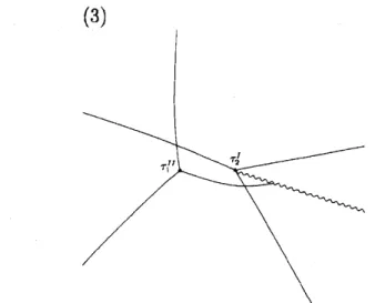
emanating from $\tau_{2}^{\mathrm{I}\mathrm{I}}$ i$\mathrm{n}$ Figure 1(2), i.e.,

on

the

second sheet of$\mathcal{R}$ (cf. Figure 3).

$\tau_{1}^{\mathrm{I}}$ ’

$\prime\prime\prime$

$\tau_{2}^{\mathrm{I}\mathrm{I}}$

$T$

Figure 3: Crossing point $t=T$ oftwo Stokes

curves on

the second sheet and

a

new

Stokes

curve

emanating from $T$

.

Here the Stokes

curve

emanating from $\mathrm{y}\mathrm{i}$ is oftype $(1, +)>(1, -)$ and defined by

(26) Irn$\int_{\tau_{1}^{\mathrm{I}}}^{t}(\nu_{1,+}-\nu_{1,-})dt=0,$

and the Stokes

curve

emanating from $\tau_{2}^{\mathrm{I}\mathrm{I}}$ is of type $(2, +)>$ $(1, +)$ and $(1,$ $-)$ >

(2, -), defined by

(27) ${\rm Im} \int_{\tau_{2}^{11}}^{t}(\nu_{2,+}-\nu_{1,+})dt={\rm Im}\int_{\tau_{2}^{11}}^{t}(\nu_{1,-}-\nu_{2,-})dt=0.$

(Concerning Stokes

curves

emanating from

a

turning point ofthe second kind, two

Stokes

curves

sit

on one

and the

same

curve

in general.) Since $t$ $=T$ lies

on

the

Stokes

curve

(26) and

(28) 2${\rm Im}$$\int_{a(t)}^{b_{1}}$

(’

$\sqrt{Q_{0}(x,t)}dx=\frac{1}{2}{\rm Im} 7_{1}^{t}\mathrm{I}(\mathrm{J}_{1,+}-\nu_{1,-})dt=0$

holds there thanks to (22),

we

find

a

simple turning point $x=a(t)$ and

a

double

since $t=T$ lies

on

the Stokes

curve

(27) and (29) 2${\rm Im} \int_{b_{1}(t)}^{b_{2}(t)}\sqrt{Q\mathrm{o}(x,t)}dx$

$={\rm Im} \int_{\tau_{2}^{11}}^{t}(\nu_{2,+}-\nu_{1,+})dt={\rm Im}\int_{\tau_{2}^{11}}^{t}(\nu_{1_{1}-}-\nu_{2,-})$dt

$=0$

holdsthere, thedouble turningpoint $r=b_{1}(t)$ and another double turningpoint$x=$

$b_{2}(t)$

are

connected by

a

Stokes

curve

at $t=T.$ Thus, if

we

draw the configuration

ofStokes geometry of (the first equation (6.a) of) the underlying Lax pair $(L_{\mathrm{I}})_{2}$ at

$t$ $=T,$

we

should find that the three turning points$x=a(t)$, $x=b_{1}(t)$ and $x=b_{2}(t)$

are

simultaneouslyconnected by Stokes

curves

of $(L_{\mathrm{I}})_{2}$

.

Actually, with the helpof

a

computer,

we

find the following Figure 4 which describes theconfiguration ofStokes

curves

of $(L_{\mathrm{I}})_{2}$ at $t=T$ The

new

Stokes

curve

emanating from $T$ is then defined $\underline{|}$

$a$

$b_{1}$

$b_{2}$

$\backslash$

Figure 4: Stokes

curves

of $(L_{\mathrm{I}})_{2}$ at $t=T.$

as a curve on

which the two ‘distant’ turning points $x=a(t)$ and $x=b_{2}(t)$

are

connected by

a

Stokes

curve

of $(L_{\mathrm{I}})_{2}$

.

As

a

matter of fact, the relation

(30) 2${\rm Im} \int_{a(t)}^{b_{2}(}$

’

$\sqrt{Q_{0}(x,t)}dx=$ $\mathrm{r}$${\rm Im} \int_{T}^{t}(\nu_{2,+}-\nu_{2,-})$dt

holds (cf. [KKNT, Theorem 4.1]) and hence

on

the

new

Stokes

curve

in question

we

have

(31) ${\rm Im} \int_{a(}^{b}2\mathrm{j}’)$ $\sqrt{Q_{0}(x,\mathrm{t})}dx=0,$

as

thedefinition of the

new

Stokes

curve

is given by vanishingof the right-hand side

5

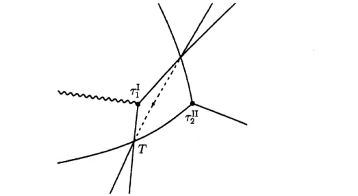
Virtual turning

points

In this section

we

discuss

a

new

Stokes

curve

from the viewpoint ofvirtual turning

points;

we

first introduce the notion of

a

“virtual turning point” for $(ffl)_{m}$ and

consider

a new

Stokes

curve as a

Stokes

curve

emanating from

a

virtual turning

point.

For the illustration of

our

discussion let

us

continue discussing the fourth order

Painlev\’e-I equation $(ffl)_{2}$ andparticularlythe

new

Stokes

curve

of itpassingthrough

the crossing point $T$ ofStokes

curves on

the second sheet. We first recall that,

as

was

explained in the preceding section, the

new

Stokes

curve

in question is defined

by (31). Note that (22) and (23) (cf. (28) and (29) also) lead to

(22) 2 $76t7^{(t)} \sqrt{Q_{0}(x,t)}dx=2\int_{a(t)}^{b_{1}}(’$ $\sqrt{Q_{0}(x,t)}dx+2\int_{b_{1}(t)}^{b_{2}(t)}\sqrt{Q_{0}(x,t)}dx$

$=2$ $\int_{\tau_{1}^{1}}^{t}(\nu_{1,+}-\nu_{1,-})dt+\int_{\tau_{2}^{\mathrm{I}\mathrm{I}}}^{t}(\nu_{2,+}-\nu_{1,+})dt$

$= \frac{1}{2}(\int_{\tau_{2}^{11}}^{t}(\nu_{2,+}-\nu_{1,+})dt+\int_{\tau_{1}^{1}}^{\mathrm{t}}(\nu_{1,+}-\nu_{1,-})d\mathrm{t}+\int_{\tau_{2}^{\mathrm{I}1}}^{t}(\nu_{1,-}-\nu_{2,-})$

dt)

Letting $I(t)$ denote the quantity in the most right-hand side of (32),

we

now

pick

up

a

point $t=\omega$ satisfying

(33) 2$\int_{a(}^{b}$

ij’)

$\sqrt{Q_{0}(x,\omega)}dx=I(\omega))=0.$

(The existence ofsuch

a

point $\mathrm{t}=\omega$has been already discussed in [KKNT, Remark

4.1].) Then

we

obtain

(34) 2$\int_{a(t)}^{b_{2}(t)}\sqrt{Q_{0}(x,t)}dx$

$=I(t)-I(\omega)$

$= \frac{1}{2}(\int_{\omega}^{t}(\nu_{2,+}-\nu_{1,+})dt+\int_{\omega}^{t}(\nu_{1_{\mathrm{I}}+}-\nu_{1,-})d\mathrm{t}+\int_{\mathrm{t}d}^{t}(\nu_{1,-}-\nu_{2,-})dt)$

$= \frac{1}{2}\int_{1d}^{t}(\nu_{2,+}-\nu_{2,-})$dt.

Hence the

new

Stokes

curve

passing through $T$

can

be described also by

(35) ${\rm Im} \int_{\omega}^{t}(’ 2,+-\nu_{2,-})dt=0,$

Remark 2. The point $t=\omega$ can be regarded as a virtual turning point of the

$\mathrm{R}6\mathrm{c}\mathrm{h}\mathrm{e}\mathrm{t}$ derivative $(\Delta P_{\mathrm{I}})_{2}$ in the following

sense:

For

a

higher order linearordinary differential operator with

a

large parameter $\eta$

a

virtual turning point is defined as (the projection onto the space of independent

variable, i.e., the $t$-space in the

case

of $(\Delta P_{\mathrm{I}})_{2}$, of)

a

self-intersection point ofthe

bicharacteristic

curve

of its Borel transform with respect to the large parameter $\eta$

(cf. [AKT]). In the

case

of $(\Delta P_{\mathrm{I}})_{2}$, if

we

ignore the singularities in the lower order

terms of $(\Delta P_{\mathrm{I}})_{2}$, the bicharacteristic

curve

is locally given by

(36) $\{(t, y)\in G;y=\int^{t}\nu_{g,*}|d\mathrm{t} \}$ ($j=1,2$ and $*=\pm$)

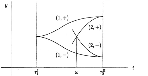
(cf. $[\mathrm{T}$, Section 3.2]). Note that the

$y$-component of the bicharacteristic

curve

is

determined only up to

an

additive constant. Now at the turning point $\tau_{1}^{\mathrm{I}}$ two

branches

(37) $(t, \int_{\tau_{1}^{1}}^{t}\nu_{1,+}d\mathrm{t})$ and $( \mathrm{t}, \int_{\tau}i \nu_{1,-}dt)$

of the bicharacteristic

curve

meet

as

$\tau_{1}^{\mathrm{I}}$ is

a

simple turning point of$(\Delta ffl)_{2}$

.

(To be

more

precise, the twobranches form

a

cusp

near

4,

while the bicharacteristic strip,

i.e., the lift of the bicharacteristic

curve

to the cotangent space, defines

a

smooth

curve

there.) These two branches (37)

are

prolongedto

a

neighborhood of the other

turning point $\tau_{2}^{\mathrm{I}\mathrm{I}}$ and have the following expression there:

(38) $(t, \int_{\tau_{1}^{1}}^{\tau}"\nu_{1,+}dt+\int_{\tau_{2}^{\mathrm{I}1}}^{t}\nu_{1,+}dt)$ and $(t, \int_{\tau_{1}^{1}}^{\tau \mathrm{I}^{1}}\nu_{1,-}dt+\int_{\tau_{2}^{\mathrm{I}1}}^{t}\nu_{1,-}dt)$

.

Then, by a similarreasoning,

we

find that the two branches (38) respectively meet

the following branches at $\tau_{2}^{\mathrm{I}\mathrm{I}}$:

(39) $( \mathrm{t}, \int_{\tau}i^{2}11 \nu_{1,+}dt +\int_{\tau}i_{1} \nu_{2,+}d\mathrm{t})$ and $(t, \int_{\tau}"\nu_{1,-}clt+\int_{\tau_{2}^{1\mathrm{t}}}^{t}\mathrm{i}’ \mathrm{i},-dt)$.

Now

we

consider

a

crossing point ofthe two branches given by (39) (cf. Figure 5).

Such

a

crossing point (i.e.,

a

self-intersection point of the bicharacteristic curve) is

determined by

(40) $\int_{\tau_{1}^{1}}^{\tau_{2}^{11}}\nu_{1,+}dt+\int_{\tau_{2}^{11}}^{t}\nu_{2,+}dt$ $= \int_{\tau_{1}^{1}}^{\tau_{2}^{\mathrm{I}\mathrm{I}}}\nu_{1,-}dt+\int_{\tau_{2}^{1\mathrm{I}}}^{t}\nu_{2,-}dt,$

which is equivalent to$I(t)=0.$ Hence the point$t=\omega$

can

be regarded

as a

a

virtual

$y$ $i$ “ $\mathrm{i}|$ : _{$(1, +)$ .}$\cdot$ ‘ $|!||,\cdot$ $(2, +)$

.

$|||$ “ $||$ . $(2,$$-)$ $||$ . $(1,$ $-)$ $i||$

.

$|$

.

$\mathrm{t}$ . $|||||||$ $\tau_{1}^{\mathrm{I}}$ – $\tau_{2}^{\mathrm{I}\mathrm{I}}$ $-$

Figure 5: Schematic illustration of the bicharacteristic

curve

of $(\Delta P_{\mathrm{I}})_{2}$

.

(The

symbol $(1, +)$ etc. designate the branch given by (36) with $(j, \mathrm{c})$ $=(1, +)$ etc.)

In view of Remark 2, it is appropriate to call the point $t=\omega$ to be

a

”virtual

turning point” of $(P_{\mathrm{I}})_{2}$. One important point here is that $t=\omega$ is defined not only

by $I(\omega)=0$ but also by the equation 2$\int_{a(\omega)}^{b_{2}(\omega)}\sqrt{Q_{0}(x,\omega)}dx=0$ which is equivalent

to $I(\omega)=0,$ that is, $t=\omega$ is defined in terms ofthe integral associated with the

underlying Lax pair $(L_{\mathrm{I}})_{2}$. Having this fact in mind,

we

define

a

virtual turning

point of $(P_{\mathrm{I}})_{m}$ by using the underlying Lax pair $(L_{\mathrm{I}})_{m}$ in the following

manner:

Definition 3. Let $*_{k}(t))(k=1,2)$ be arbitrarily chosen two turningpoints of (the

first equation (6.a) of) the Lax pair $(L_{\mathrm{I}})_{m}$ (i.e., *7(t) $=a$(t)

or

$b_{j}(t)$), and let $C_{t}$ be

an

arbitrarily chosen path (in the $x$-space) connecting $*$a(t) and $*_{2}(t)$

.

Then

a

point

$t=\omega$ satisfying (41) $\int_{*_{2(\{v)}}^{*_{1}(\omega}$ , $)$ along $c_{\omega}\sqrt{Q_{0}(x,\omega)}dx=0$

is called

a

virtual turning point of $(P_{\mathrm{I}})_{m}$

.

Remark 3. In the

case

of the Painlev6-I hierarchy,

as

there exists only

one

simple

turning point, the number of possible paths $C_{t}$ in (41) is finite. Furthermore, since

$\sqrt{Q_{0}(x,t)}$

can

be explicitly integrated (with respect to $x$) like

(42) $\int^{x}\sqrt{Q_{0}}dx=$ (apolynomial in $x$) $\cross\sqrt{x-a(t)}$

in view of (20), for each choice of $C_{t}$ (the square of) (41) becomes of the form

(43) $F(b_{j}, \mathrm{i}_{1,0})$ $=0$

or

$G(b_{j}, b_{j’},\hat{u}_{1,0})$ $=0$

according

as

$(*_{1}(t), *_{2}(t))=(b_{j}(\mathrm{t}), a(t))$

or

$(b_{j}(t), b_{\mathrm{j}’}(t))$,where $F(X,u)$ and$G(X, \mathrm{Y}, u)$

$U_{0}(x, t)=0$ (or,

more

precisely,

a

root of $U_{0}(x,\hat{u}_{1,0})$ $=0$ since the $t$-dependence of $U_{0}$

comes

only from its$\hat{u}_{j}$,0-dependence) , we thus find that, in order to seek for

a

vir-tual turning point of $(P_{\mathrm{I}})_{m}$, it is sufficient to solve the following system ofalgebraic

equations

(44) $F(X, u)=U_{0}(X, u)=0$

or

$G(X, \mathrm{Y}, u)=U_{0}(X, u)=U_{0}(\mathrm{Y}, u)=0$

(where

we

put $X=b_{j}$, $\mathrm{Y}=b_{j’}$ and $t$) $=\hat{u}_{1,0})$

.

Such

a

system

can

be algebraically

solved by using the resultant. Hence

we

conclude that there exist finitely many

virtual turning points in the

case

of $(P_{\mathrm{I}})_{m}$

.

We also define

a

new Stokes curve emanating from a virtual turning point

as

follows:

Definition 4. Let $t=\omega$ be

a

virtual turning point of $(P_{\mathrm{I}})_{m}$

.

(i) When $\omega$ is defined by (41) with $*_{1}$$(t)=b_{j}(t)$ and *2(t) $=a(\mathrm{t})$,

we

define

a new

Stokes

curve

emanating from $\omega$ by

(45) ${\rm Im} 7^{t}(\nu_{j,+}-\nu_{j,-})dt=0.$

(ii) When $\omega$ is defined by (41) with 11$(t)=b_{j}(t)$ and *2(t) $=b_{j’}(t)(j\neq j’)$,

we

define

a new

Stokes

curve

emanating from$\omega$ by

(46) ${\rm Im} \int_{\omega}^{t}(\nu_{j,+}-\nu_{j’,\pm})dt={\rm Im}\int_{\omega}$

’

$(\nu_{j’,\mp}-\nu_{j,-})dt=0,$

where we take $+$ sign in the first term and – sign in the second term (resp. – sign

in the first term and $+$ sign in the second term) if $C_{\omega}$ does not

cross

(resp. does

cross)

a

cut to define $\sqrt{Q_{0}(x,\omega)}$

.

A

new

Stokes

curve

defined by (45) (resp. (46)) is called

a new

Stokes

curve

of

type $(j, +;j, -)$ (resp. of type ($j,$ $+$;$j’,$ $\pm$) and $(j$, -;$j’,$ $\mp)$). (The type of

a

virtual

turning point is defined in

a

similar manner.)

In parallel with Proposition 2, we then obtain the following Proposition 4,

a

counterpart of the relations (22) and (23), for

a

virtual turning point and a

new

Stokes

curve

emanating from it:

Proposition 4. Let $t=\omega$ be

a

virtual turning point

of

$(P_{\mathrm{I}})_{m}$. Then we have the

following relations:

(i) When$\omega$ is

defined

by (41) $with*_{1}(t)=b_{j}(t)$ and*2(t) $=a(t)$,

(47) $\frac{1}{2}\int_{\omega}^{\mathrm{t}}(l_{j,\mathit{4}}-\nu_{j,-})dt=2\int_{a(}^{b}$

3z

holds, where the integral

_of

the right-hand side

_of

(47) should be taken along the path

$C_{t}$ that appears in the

definition of

$\omega$.

(ii) When $\omega$ is

defined

by (41) $with*_{1}(t)$ $=b_{j}(t)$ and*2$(t)=b_{j’}(t)(j\neq j’)$,

(48) $\int_{\omega}^{t}(\nu_{j,+}-\nu_{j’,\pm})dt=\int_{\omega}^{t}(\nu_{j’,\mp}-\nu_{j,-})dt=2\int_{b_{j},t)}^{b_{j}(t)}.\sqrt{Q_{0}(x,t)}$dx,

holds, where the integral

_of

the right-handside should be taken along the path $C_{t}$

as

in $(i)_{f}$ and the sign $\mathrm{f}$ and

$\mathrm{F}$

are

chosen in the

same

way as in

Definition

4, (ii).

Proof

Theproofisessentiallythe

same as

that ofProposition 2 (cf. [KKNT,

PropO-sition 2.1.4]); to prove (i), let

us

consider the $t$-derivative of the right-hand side of

(47). Since both endpoints $x=b_{j}(t)$ and $x=a(t)$ of the integral

are zeros

of $Q_{0}$,

we

find

(49) $\frac{\partial}{\partial \mathrm{t}}(2\int_{a(}^{b}$

j

$)$

(’

$\sqrt{Q_{0}(x,t)}$dx

)

$=2 \int_{a(t)}^{b_{j}(t)}\frac{\partial}{\partial \mathrm{t}}ndx$

.

Here,

as

is proved in [KKNT, Proposition 2.1.2],

(50) $\frac{\partial}{\partial t}\sqrt{Q_{0}(x,t)}=\frac{\partial}{\partial x}\sqrt{x+2\hat{u}_{1,0}}$

holds. It then follows from (21) that

(51) $\frac{\partial}{\partial t}(2\int_{a(t)}^{b_{f}(t)}\sqrt{Q_{0}(x,t)}dx)=2\int_{a(t)}^{b_{j}(t)}\frac{\partial}{\partial x}\sqrt{x+2\hat{u}_{1,0}}dx$

$=2\sqrt{x+2\hat{u}_{1,0}}|_{x=b_{j}(t)}$

$= \nu_{j,+}=\frac{1}{2}(’ j,+-\nu_{j,-})$

.

As $\int_{a(\omega)}^{b_{f}(\{d)}\sqrt{Q_{0}}dx=0$holdsbythedefinition of$\omega$, integrating(51) from $\omega$to$\mathrm{t}$verifies

(47). In

a

similar

manner

we can

prove (ii) also. $\square$

Remark 4. In labeling the characteristic roots $\nu_{j,\pm}$ of$C_{0}$,

we

implicitly used the

Riemann surface of $\sqrt{Q_{0}}$,

or

cuts to define $\sqrt{Q_{0}}$. (See (21) and compare it with

(20).) Intuitively speaking, each characteristic root $\nu_{j,\pm}$ is attached to

a

double

turning point $r=b_{j}(t)$

on

the Riemann surface of $\sqrt{Q_{0}}$. (Thus it may be better

to

use

the notation $” x=b_{j,\pm}(t)$” from this viewpoint.) If in Definition 4 (ii)

we

consider $C_{\omega}$ to be a path

on

the Riemann surface of $\sqrt{Q_{0}}$ connecting two such

double turning points $b_{j,\pm}$ and $b_{j’,\pm}$, the choice of thesign in (46) is consistent with

this identification between $\nu_{j,\pm}$ and $b_{j,\pm \mathrm{i}}$ for example, if$C_{\omega}$ does not

cross a

cut to

define $\sqrt{Q_{0}}$, it connects _{$b_{j,+}(t)$} and _{$b_{j’,+}(t)$} (and simultaneously _{$b_{j,-}$}(t) and _{$b_{j’,-}(t)$}).

Then thechoiceof the signin (46) immediatelyfollows ffomthe above identification.

Note that, from this point of view, the ‘true’ path in Definition 4 (i) is not $C_{\omega}$, but

rather its double

cover

$\tilde{C}_{\omega}$, i.e., double

cover

(on the Riemann surface of

$\cap Q_{0}$ of

$C_{\omega}$ that connects _{$b_{j,+}(\omega)$} and

6

Complete description of the Stokes geometry

In the preceding section

we

gave the definition of virtual turning points and

new

Stokes

curves

emanating from them. As is exemplified by $(P_{\mathrm{I}})_{2}$,

we

have to take

such virtual turning points and new Stokes

curves

into account to obtain the correct

global Stokes geometryfor $(P_{\mathrm{I}})_{m}$

.

On the otherhand, Definitions 3 and 4 have given

us

sufficiently many virtual turning points and new Stokes

curves

in the following

sense:

If

_we

add all the virtual turning points and

new

Stokes

curves

given by

Definitions 3 and 4totheordinaryturningpointsand Stokes curves,

we

then obtain

a

“saturated Stokes geometry”. Here

we

say that

a

Stokesgeometry, i.e., thecollection

of (ordinary and virtual) turning points and (ordinary and new) Stokes curves, is

saturated (inthe

sense

that all thepossibilities

are

exhausted) ifeverycrossing point

of (ordinary $\mathrm{a}\mathrm{n}\mathrm{d}/\mathrm{o}\mathrm{r}$ new) Stokes

curves

in the Stokes geometry in question belongs

to

one

of the following three types: (In thedescription below the indices$j$, $k$, $l$ and

$m$

are

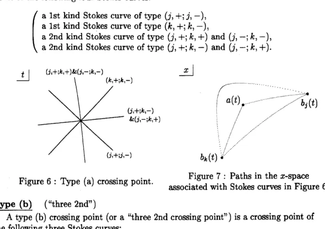
assumed to be mutually distinct.)

yp$\mathrm{e}$ (a) (“two 1st

&

two 2nd”)

A type (a) crossing point (or

a

“two 1st

&

two 2nd crossing point”) is

a

crossing

point of the following four Stokes

curves:

$\{$

a 1st kind Stokes curve oftype $(j, +;j, -)$,

a

1st kind Stokes

curve

oftype $(k, +;k,-)$,

a 2nd kind Stokes curve of type $(j, +;k, +)$ and $(j, -;k,-)$ ,

a

2nd kind Stokes

curve

oftype $(j, +\mathrm{i}k, -)$ and $(j, -;k, +)$.

$\underline{t|}$ $(j,+j,+)\ (j,-jk,-)$ $\underline{x|}$ $(k,+j,-)$ $f^{\prime’}$ $a(t)$

.

$b_{j}(t)$ $(j,+j,-)\ (j,-jk,+)$ $(j,+;j,-)$ _{$b_{k}(t)$}

.

Figure 7: Paths in the rc-space

Figure 6: Type (a) crossing point.

associated with Stokes

curves

in Figure 6.

Type (b) (“three 2nd”)

A type (b) crossing point (or

a

“three 2nd crossing point”)$)$ is

a

crossing point of

the following three Stokes

curves:

$\{$

a

2nd kind Stokes

curve

of type $(j, +;k, +)$ and $(j, -;k,-)$,

a

2nd kind Stokes

curve

of type $(k, +;l, +)$ and $(k, -;l,-)$,

(or the pattern where the sign $\pm$ associated with

an

index, say, I is interchanged

like “type $(j, +;k, +)$ and $(j, -;k, -)$, type $(k, +;l, -)$ and $(k, -;l, +)$, and type

$(j, +;l, -)$ and $(j, -;l, +)$”_). $\underline{t}|$ $\underline{x|}$ $(k,+jl,+)\ (k,-l,-)$ $b_{k}(t)$

.

$.\dot{b}_{j}.(t)$ $(j,+jk_{1}+)\ (j,-k,-)$ $b_{l}(t)$

.

Figure 9: Paths in the z-space

Figure 8:Type (b) crossing point. _{associated with Stokes}

_curves

_i

$\mathrm{n}$ Figure 8.

Type (c) $(” \mathrm{d}\mathrm{i}\mathrm{s}\mathrm{j}\mathrm{o}\mathrm{i}\mathrm{n}\mathrm{t}")$

A type (c) crossing point (or

a

“disjoint crossing point”) is

a

crossing point of

the following two Stokes

curves:

ype (c-1)

$\{$

a

1st kind Stokes

curve

oftype

$(j, +;j,-)$,

a

2nd kind Stokes

curve

oftype $(k, +;l, +)$ and $(k, -;l_{3} -)$,

’ $l$ $x$

.

$t$ $t$

Figure 11 :Paths associated with Stokes

Figure 10 : Type (c-1) crossing point.

_curves

in Figure 10.

yp$\mathrm{e}$ (c-2)

$\{$ a2nd kind Stokes

curve

oftype

$(j, +;k, +)$ and $(j, -;k,-)$,

a2nd kind Stokes

curve

of type $(l, +;m, +)$ and $(m, -;l,-)$,

$\underline{t|}$ $\underline{x|}$ -$\cdot$ $b_{j}$$(t)$ $k$ $b_{k}(t)$ $\prime\prime\prime\nu\wedge$ $b_{l}(t)$ $b_{m}(t)$

.

Figure 13:Paths associated with Stokes

Figure 12 : Type (c-2) crossing point.

curves

in Figure 12.

Let

us

explain the

reason

why

we

obtain a saturated Stokes geometry if

we

consider all the virtual turning points and

new

Stokes

curves

together with the

ordinaryturning points and Stokes

curves.

A key point is that the above local data

near

acrossing point of Stokes

curves

in the$t$-space

can

be translatedintothe global

data in the $x$-space. In fact,

as

is claimed in Proposition 2

or

4,

a

path (in the

x-space) connecting two turning points of theunderlying Lax pair $(L_{\mathrm{I}})_{m}$ is associated

with each (ordinary

or

new) Stokes

curve

of$(P_{\mathrm{I}})_{m}$ via theintegralrelations like (22),

(23)$)$ $(47)$

or

(48). Thus, if

we

take

a

crossing point of two (ordinary

$\mathrm{a}\mathrm{n}\mathrm{d}/\mathrm{o}\mathrm{r}$ new)

Stokes curves,

we

are

given two such paths in the $x$-space associated with them and

four turning points of $(L_{\mathrm{I}})_{m}$ being endpoints of these two paths. Then, concerning

the combination of the four endpoints,

we

have the following three

cases:

(1) The two paths share

one

endpoint and consequently

we are

given three

end-points, amongwhich

a

simple turning point is included.

(2) The two paths share

one

endpoint and consequently

we are

given three

end-points, all ofwhich

are

double turning points.

(3) The four endpoints (turning points) are mutually disjoint.

The

case

(1) corresponds to

a

type (a) crossing point: At such

a

crossing point three

turningpoints $a(t)$, $b_{j}$(t) and $b_{k}(t)$

are

relevant in the $\mathrm{z}$-space. Then,

as

a

path of

integration for $\sqrt{Q_{0}}$ connecting two of them,

we

may consider four possible paths,

as

is shown in Figure 7. (Notethat $\sqrt{Q_{0}}$ is holomorphic at

a

double turning point,

while

a

simple turningpoint is

a

square-roottypesingular point of !.) Since the

imaginarypart of the integral of$\sqrt{Q_{0}}$along two ofsuch fourpossible paths vanishes

by the assumption thatthepoint inquestion is

a

crossingpointoftwo Stokes curves,

the imaginary part of the integral along all of these four paths should vanish. As

we

have exhaustively taken into account all the possible paths in defining virtual

turningpoints and

new

Stokes curves, this

means

that four Stokes

curves

must

cross

at the point in question and hence

we

conclude that such

a

crossing point is

a

type

(a) crossing point. By

a

similar argument

we can

also confirm that the

case

(2)

all the (ordinary and virtual) turning points and (ordinary and new) Stokes curves,

only the three types ofcrossing points of Stokes

curves

may appear.

Remark 5. For $(P_{\mathrm{I}})_{2}$ neithertype (b)

nor

type (c) crossing points appear, since the

underlying Lax pair $(L_{\mathrm{I}})_{2}$ has just two double turning points. Similarly type (c-2)

crossing points do not appear for $(P_{\mathrm{I}})_{3}$.

In this way, by adding virtual turning points and

new

Stokes curves,

we

obtain

a

saturated Stokes geometry of $(ffl)_{m}$

.

However, to obtain a “complete Stokes

ge-ometry” of $(ffl)_{m}$, i.e., its correct global Stokes geometry,

we

still need to discuss

the “effectiveness”

or

“activity” ofStokes

curves.

That is,

on

each portion ofStokes

curves we

have to check whether the degeneracy of Stokes geometry of the

under-lying Lax pair $(L_{\mathrm{I}})_{m}$ does really

occur or

not. (On each Stokes

curve

we

have the

relation

(52) ${\rm Im} 7_{1}^{*}2_{t}\mathrm{j}$

’

$\sqrt{Q_{0}}dx=0$

with

some

turning points $*_{1}(t)$ and *2(l) of $(L_{\mathrm{I}})_{m}$, but (52) does not necessarily

imply the degeneracy of Stokes geometry of $(L_{\mathrm{I}})_{m}$. See [AKT, p.80] and [KKNT,

Remark 4.1].)

Concerning the problem of activity of Stokes curves,

we

first note the following

Proposition 5. A

nern

Stokes curve is not active

near

a virtual turning $point_{f}$ that

is,

no

degeneracy

_of

the Stokes geometry

_of

$(L_{\mathrm{I}})_{m}$ occurs on a

nern

Stokes

curve near

a

virrual turningpoint.

Proof.

Assume that

a

virtual turning point $t=\omega$ is not

an

ordinary turning point

and that it is defined by

(53) $\int_{*}i$ ’

$\sqrt{Q_{0}}\mathrm{b}$ _$=0$

with

some

turning points $*_{1}$ and $*_{2}$ of $(L_{\mathrm{I}})_{m}$

.

Ifthe degeneracy of Stokes geometry

of $(L_{\mathrm{I}})_{m}$

were

to

occur on a new

Stokes

curve

emanating from $t=\omega$, the turning

points $*_{1}$ and $*_{2}$ should be connected by

a

Stokes

curve

7 of $(L_{\mathrm{I}})_{m}$ at $t=\omega$. Since

(54) $\int_{*_{2}}^{x}\sqrt{Q_{0}}\mathrm{r}x$

is

a

real-valued monotone function (of $x$)

on

$\gamma$, it then follows bom (53) that $*1$

should coincide with $*_{2}$

.

This

means

that $t–$ \mbox{\boldmath$\omega$} should be

an

ordinary turning

point, contradicting the assumption. $\square$

Hence,

as

in the

case

of higher order linear equations, the portion of

a new

Stokes geometry (i.e., be drawn by

a

dotted line). On the other hand, in view of

Proposition 2,

we

should keep solid the portion of

an

ordinary Stokes

curve

near

an

ordinary turningpoint. Thus the activity ofStokes

curves

is completelydetermined

near

turning points.

Note that the degeneracy of Stokes geometry of $(L_{\mathrm{I}})_{m}$, i.e., the existence of a

Stokes

curve

connecting two turning points, may be resolved only when another

turning point of $(L_{\mathrm{I}})_{m}$

comes

across

the Stokes

curve

in question. Since such

a

phenomenon

occurs

only at a crossing point of Stokes

curves

of $(ffl)_{m}$,

we

find that

the activity of

a

Stokes

curve

of $(P_{\mathrm{I}})_{m}$ changes only at

a

crossing point of Stokes

curves.

Thus, from

now

on,

we

consider classification ofall the ’admissible’ patterns

forthe activityofStokes

curves

at each type ofcrossing points. Let

us

first discuss

a

type (a) (i.e., two 1st

&

two 2nd) crossing point ofStokes

curves.

At such

a

crossing

point three turning points $a(t)$, $b_{j}(t)$ and $b_{k}(t)$ of $(L_{\mathrm{I}})_{m}$

are

relevant in the z-space

(cf. Figure 7). Concerning the

occurrence

of degeneracy of the Stokes geometry of

$(L_{\mathrm{I}})_{m}$,

we

have the following three

cases:

(i) No pair of the three turning points is connected by

a

Stokes

curve

of$(L_{\mathrm{I}})_{m}$

.

(ii) Only two of them are connected by a Stokes

curve

of $(L_{\mathrm{I}})_{m}$

.

(iii) All of them

are

connected by (two) Stokes

curves

of $(L_{\mathrm{I}})_{m}$.

In Case (i) all Stokes curves of $(ffl)_{m}$ passing through the crossingpoint in question

are

inactive (i.e., should be drawn by

a

dotted line), while only

one

Stokes

curve

is

active and the others

are

inactive in Case (ii). Case (iii)

can

be further classified

into the following three subcases:

Case (iii-l) Case (iii-2)

Case (iii-3) $\underline{x|}$

Figure

14

: Stokes geometry of $(L_{\mathrm{I}})_{m}$ in Case (iii).

All of these three subcases have already been discussed in [KKNT, Section 4];

Cases (iii-l) and (iii-2)

are

Lax-adjacent crossing points and Case (iii-3) is

non-Lax-adjacent. The corresponding admissible patterns for the activity of Stokes

curves

of

$(ffl)_{m}$ will be given in Figure 15 below. Thus the classification of all the admissible

patterns at

a

type (a) crossing point is

now

completed.

In a similar

manner we can

classify all the admissible patterns also at type (b)

and (c) crossing points. The followingis

a

list of all the admissible patterns for the

activity of Stokes

curves

at each type of crossing points:

List of the admissible patterns for the activity of Stokes

curves

at each

type of crossing points

Type (a) (“two 1st

&

two 2nd”)

(i) All

curves are

dotted.

(ii) Only

one curve

is solid, the others

are

dotted.

(iii) (See below.)

Case (iii-l) Case $(\mathrm{i}\mathrm{i}\mathrm{i}- 1)’$

$\underline{t|}$

$\lambda_{1}^{k}k$

$\underline{t|}$

Case (iii-2) Case (iii-3) $\underline{t|}$

$*_{\iota}’/$

$*1//$ $k2$ $\underline{t|}$ $|$

Figure 15 : Admissible patterns at

a

type (a) crossing point (in Case (iii)).

$\mathrm{y}\mathrm{p}\mathrm{e}$ $(\mathrm{b})$ $($$(” \mathrm{t}\mathrm{h}\mathrm{r}\mathrm{e}\mathrm{e} 2\mathrm{n}\mathrm{d}")$

(i) All

_{curves are}

dotted.

(ii) Only

one curve

is solid, the others

are

dotted.

(iii) (See below.)

Case (iii-l) Case (iii-2)

$\underline{t|}$ $\underline{t|}$ $(j_{1}+|.l,+)\ (j,-;l,-)|$

$k$

$k$

$|$ $|$

Figure 16 : Admissiblepatterns at

a

type (b) crossing point (in Case (iii)).

Type (c) $(” \mathrm{d}\mathrm{i}\mathrm{s}\mathrm{j}\mathrm{o}\mathrm{i}\mathrm{n}\mathrm{t}")$

(i) All

curves are

dotted.

(ii) Only

one

curve

is solid, the others

are

dotted.

(iii) Both

curves are

solid.

Remark 6. As in the description ofeach type ofcrossing points, i.e.,

as

in Figures

6, 8, 10 and 12, the combination of the types of Stokes

curves

is not completely

listed and

some

interchange of the sign $\pm$ is allowed in Figures 15 and 16. In these

figures the placement ofStokes

curves

is not specified, either.

By the

same

reasoning

as

in [KKNT, Remark 4.1]

we

can

verify that

a

point

an

ordinary

or

new Stokes

curve

of $(P_{\mathrm{I}})_{m}$. Hence the “complete Stokes geometry”

of $(P_{\mathrm{I}})_{m}$, i.e., the collection of points where the degeneracy of Stokes geometry

of the underlying Lax pair $(L_{\mathrm{I}})_{m}$ is observed, should consist of the (ordinary and

virtual) turning points and the (ordinary and new) Stokes

curves.

Furthermore, in

the complete Stokes geometry the pattern of the activity of Stokes

curves

at each

crossing pointshouldnecessarily belong tothe above list. Thus,

as

theprocedurefor

determining the complete Stokes geometry of $(P_{\mathrm{I}})_{m}$,

we

can

propose the following:

Procedure for determining the complete Stokes geometry

1’) Draw the Stokes

curves

emanating from ordinary turning points.

2’) Locateall the virtualturningpointsanddrawthe

new

Stokes

curves

emanating

from them.

3’) The portion of

a new

Stokes

curve

containing

a

virtual turning point should

be ignored in the Stokes geometry (i.e., be drawn by

a

dotted line).

4’) The portion of

an

ordinary Stokes

curve

adjacent to

an

ordinaryturningpoint

should be kept solid.

5’) We determine the activity ofeach portion ofStokes

curves so

that, in addition

to $3^{\mathrm{o}}$) and 4’), the patternofthe activityat every (type (a), (b)

or

(c)) crossing

point of Stokes

curves

may belong to the above list.

$6^{\mathrm{o}})$ The complete Stokes geometry is then given by the collection of the turning

points and solid (active) portions of Stokes

curves

determinedby $5^{\mathrm{o}}$).

If the activity ofeach portion of Stokes

curves

is uniquely determined in

a

globally

consistent manner by 5’), the Stokes geometry thus obtained is nothing but the

complete Stokes geometry. For example,

as we

shall

see

in what follows,

we can

obtain the complete Stokes geometry of $(P_{\mathrm{I}})_{2}$ and that of $(P_{\mathrm{I}})_{3}$ by following the

above Procedure.

Example 1 (revisited). In the

case

ofthe 4th order Painlev\’e-I equation $(ffl)_{2}$,

if

we

add virtual turning points and

new

Stokes

curves

to ordinary turning points

and ordinary Stokes curves,

we

obtain Figure 17. (In Figure 17 (and in Figures 18,

20 and 21 below

as

well) virtual turning points

are

denoted by small dots, while

ordinary turning points

are

denoted by largedots.) Furthermore, using $3^{\mathrm{O}}$), $4^{\mathrm{o}}$) and

$5^{\mathrm{o}})$ of the above Procedure,

we can

uniquelydetermine the activityof each portionof

Stokes curves,

as

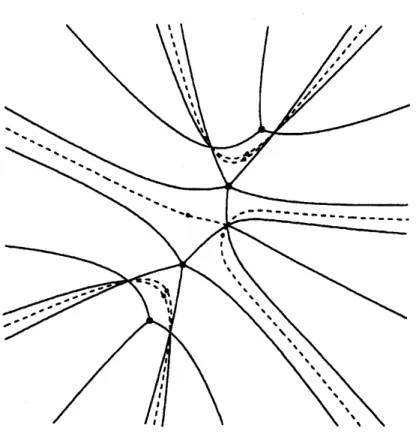
is shown in Figure 18. Thus Figure 18 gives acompletedescription

Figure 17 : Saturated Stokes geometry of $(P_{\mathrm{I}})_{2}$ in the w-plane. 1 $\prime\prime$

.

1 1 $\prime\prime\prime$ $\iota$ $\iota_{1\backslash }$ $\prime\prime\prime$ $\backslash \backslash$

$\backslash \backslash \backslash$

$\backslash$ $\backslash$

$\backslash \backslash$

$.\backslash \backslash -\sim*$ $\backslash \backslash$ $\backslash \backslash$ $\backslash \backslash$ $\backslash \backslash$ – $\backslash$ $\prime\prime---rightarrow---\cdot$ $\vee\sim\backslash$ ’ $\backslash$ $\backslash$ $\prime\prime\prime\prime\prime\prime’\sim$ ’

$\backslash \sim\backslash \backslash \grave{\grave{\tau}}_{1}$

$\backslash$ $\backslash$ $\prime\prime\prime$ ’ $\backslash$ $\backslash$ $\backslash$ ’ $\backslash$ $\backslash$ $\backslash$

$\backslash \backslash \backslash$ $\iota$

Example 2. (6th order Painlev\’e-I equation)

$(P_{\mathrm{I}})_{3}$ $u^{(6)}=\eta^{2}(28uu^{(4)}+56u’u^{(3)}+42(u’’)^{2})-\eta^{4}(280u^{2}u’’+$ $280\mathrm{t}\mathrm{z}(u’)^{2}$

$+16c_{1}u’’)+\eta^{6}(280u^{4}+96c_{1}u^{2}-64c_{2}u-32c_{1}^{2}+64t)$

.

Similarlyto the

case

of$(P_{\mathrm{I}})_{2}$

we

can

take$u=\hat{u}_{0}$

as a

globally uniformizingparameter

of its Riemann surface II (cf. [NT]). Figure19 describesthe configuration ofordinary

Stokes

curves

of $(ffl)_{3}$ in the u-plane.

Just like $(ffl)_{2}$, adding virtual turningpoints and

new

Stokes

curves

to Figure 19

and using 3’), $4^{\mathrm{o}}$) and 5’) of the above Procedure to determine the activity of each

portion of Stokes curves,

we

obtain Figure 20 and Figure 21. Thus Figure 21 gives

a complete description of the global Stokes geometry for $(P_{\mathrm{I}})_{3}$

.

Figure 19 : Stokes

curves

of $(ffl)_{3}$ (in the u-plane).

Remark 7. The procedure for determining the complete Stokes geometry

can

be

applied in principle to other (hierarchies of) higher order Painlev! equations,

as

long

as

their underlying Lax pairs

are

2 $\mathrm{x}2$ linear systems. There are, however,

some

diiBculties to obtain

a

complete description ofthe global Stokes geometry for

Figure 20 : Saturated Stokes geometry of$(ffl)_{3}$

.

classification (of the types) of crossing points ofStokes

curves

in asaturated Stokes

geometry may not be complete in general, and another

one

is that infinitely many

virtual turningpointsmay appearforhigher orderPainlev6 equations (except forthe

Painleve-I hierarchy). Both difficulties originate from the fact that the underlying

Lax pair has several simple turning points and consequently there exist nontrivial

period integrals $\oint\sqrt{Q_{0}}$ S. Among them the second difficulty is

more

serious;

as

in

the

case

ofhigherorder linear equations, howto dealwithinfinitelymanyredundant

virtual turning points is

an

important open problem.

Acknowledgement

This research issupportedinpart byJSPS Grant-in-AidNo. 14340042,No. 15740088

Figure 21 : Complete Stokes geometry of $(ffl)_{3}$.

References

[AKT] T. Aoki, T. Kawai and Y. Takei: New turning points in the exact WKB

analysisforhigherorderordinarydifferentialequations,Analyse alg\’ebrique

desperturbationssinguliferes, I; M\’ethodesr\’esurgentes, Hermann, 1994, pp.

69-84.

[BNR] H. L. Berk, W. M. Nevins and K. V. Roberts: New Stokes’ line in WKB

theory, J. Math. Phys., 23(1982), 988-1002.

[GP] P.R. Gordoa and A. Pickering: Nonisospectral scatteringproblems: A key

[KKNT] T. Kawai, T. Koike, Y. Nishikawa and Y. Takei: On the Stokes geometry

ofhigher order Painleve’ equations, RIMS Preprint No. 1443, 2004.

[KT1 T. Kawai and Y. Takei: WKB analysis of Painlev6 transcendents with a

large parameter. $\mathrm{I}$, Adv. Math., 118(1996), 1-33.

[KT2] –: Algebraic Analysis of Singular Perturbations, Iwanami, Tokyo,

1998. (In Japanese. An English translation is to be published by A.M.S.)

[K] N. A. Kudryashov: Thefirst and second Painlev? equations of higher order

and

some

relations between them, Phys. Lett. $\mathrm{A}$, 224(1997), 353-360.

[KS] N. A. Kudryashov and M. B. Soukharev: Uniformization and

transcen-dence of solutions for the first and second Painlev6 hierarchies, Phys. Lett.

$\mathrm{A}$, 237(1998), 206-216.

[N1] Y. Nishikawa: WKB analysis of $ffl_{\mathrm{I}^{-}}P_{\mathrm{I}V}$ hierarchies, Master Thesis, Kyoto

Univ., 2003. (In Japanese.)

[N2] –: Towards theexact WKB analysis of$ffl_{\mathrm{I}^{-}}ffi$hierarchies. Preprint.

[NT] Y. Nishikawa and Y. Takei: On the structure of the Riemann surface in

the Painleve’ hierarchies. In Prep.

[S1] S. Shimomura: Painleve’propertyof

a

degenerate Gamier system of

(9/2)-type and of

a

certain fourth order non-linearordinary differentialequation,

Ann. Scuola Norm. Sup. Pisa, 29(2000), 1-17.

[S2] –: On the Painlev! I hierarchy, RIMS K\^oky\^uroku, No. 1203, 2001,

pp. 46-50.

[S3] A certain expression ofthe first Painleve’ hierarchy, preprint.

[T] Y. Takei: Exact WKB analysis, and exact steepest descent method. –

A sequel to “algebraic analysis of singular perturbations” -, Sugaku,

55(2003), 350-367. (In Japanese. Its English translation will appear in