A Simple SOCP formulation of Minimization of Network Congestion Ratio (The state-of-the-art optimization technique and future development)

A

_Simple

SOCP formulation of

\mathrm{M}

而而zation

of Network

_Congestion

Ratio

Bimal Chandra

_Das,

_Eiji

Oki and Masakazu Muramatsu

Department

of Communication

_Engineering

and Informatics

The

_University

of

_{Electro‐Communications,}

_Tokyo

\mathrm{E}‐mail:

_{[email protected], [email protected], [email protected].}

1

Introduction

The networklinkutilizationrate is the ratio oftraffic flow

_through

alink and its

capacity.

Thenetwork

_congestion

ratioisthemaximumvalue of all links utiliza‐

tionrates. Whensomehnksornodesinnetwork broadcasttoomuch

information,

it causes network

congestion

and decreases the network

performance by taking

moretimetosendinformation fromsourceto

_destination,

_packet

lossor

reducing

the

_throughput

_([1]).

Howtominimize the

_congestion

ratio isan

important

affairs

of information and communication

_technology

_(ICT)

sector.

Thereare several researches onthe minimization of the network

congestion

ratio.

_Wang

and

_Wang

_[2]

_proposed

a

specific routing problem

for intemettraffic

engineering

as alinear

programming

(LP)

problem

whose

objective

istominimize

the

_congestion

ratio. Intheirwork

_they

_assuming

that the traffic demand

_{d_{pq}}

for

every

pair (p, q)

of source node pand destination node q is

exactly

known. In

fact,

duetotheexacttraffic

matrix,

_{T=\{d_{pq}\}}

this research

_provides

a

acceptable

routing

performance

than theMulti‐Protocol Label

_Switching

_(MPLS)

standard.

The traffic model which is

_exploits

theexacttraffic matrixis known as the

pipe

In this

research,

we _propose amodel based on robust

optimization

to mini‐

mizethe network

_congestion

ratio. We considersomefluctuations intheestimated

trafficdemandsof the

_pipe

model

_depending

on a_parameter

applying

robust

opti‐

mization

_technique

tobuildupsecond‐orderconeconstraintsand

finally

formulate

the

_problem

asthe SOCP model.

2

UackUone Network and Network Model

The network is

_represented

as a directed

graph

G(V, A)

, where V is the set of

vertices

_(nodes)

and A is the set of links. Let

_{Q\subseteq V}

be the setof

_edge

nodes

through

which traffic is admitted intoand

_going

outsidethenetwork. A link from

i\in Vtonode

_{j\in V\backslash \{i\}}

is denotedas

_{(i,j)\in A,}

_{i\neq j}

. Letan

edge

node

pair

of

_{p\in Q}

and

_{q\in Q}

, wherep\neq q,be denoted

by (p, q)\in W

,where W is the set

of

_{edge‐node pairs (p, q)}

.

x_{ij}^{pq}

is the

portion

oftraffic from node

p\in Q

tonode

q\in Q

routed

_through

link

_{(i,j)\in A.}

_{c_{ij}} is the

_capacity

of link

_{(i,j)\in A}

. The

network

_congestion

_ratio,

whichreferstothemaximum valueof alllinkutilization

ratesin the

_network,

is denoted

_by

r. Theadmissible trafficin the networkcanbe

maximized

_{by minimizing}

the network

_congestion

_ratio,

r. Theadmissibletraffic

is

_accepted

_uptothecurrenttraffic volume

_multiplied

_{by 1/r.}

The backbone network or network that interconnects various

pieces

of net‐

work

_{provides paths}

for the

_exchange

of informationbetween different LANsor

subnetworks. It can tie

together

diverse networks inthe same area, in different

areas,or overwideareas. A

large corporation

that has_manylocations_mayhavea

backbone networkthat ties all ofthelocations

_together.

Thenetwork

_congestion

ratioisoften takeninto consideration while

_designing

thenetwork. Tominimize

the network

_congestion

ratiowith

_routing

controlis the

_objective

of this_paper.

3

_Pipe

Model

Inthe

_pipe

_model,

the traffic demand information

_{T=\{d_{pq} : (p, q)\in W\}}

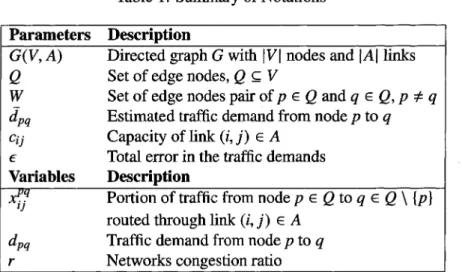
are

Table 1:

_Summary

of Notations

Parameters

_Description

G(V, A)

Directed

_graph

Gwith

_|V|

nodesand

_|A|

links

Q

Setof

_edge

nodes,

Q\subseteq V

W Setof

_edge

nodes

_pair

of

_{p\in Q}

and

_{q\in Q,}

_{p\neq q}

\overline{d}_{pq}

Estimated trafficdemand from node pto_q

c_{ij}

Capacity

of link

(i,j)\in A

$\epsilon$ Totalerrorin thetraffic demands

Variables

_Description

Portion of traffic fromnode

_{p\in Q}

to

_{q\in Q\backslash \{p\}}

ij

routed

_through

link

_{(i,j)\in A}

d_{pq}

Traffic demand from node pto_q

r Networks

congestion

ratio

formulation for the

_pipe

modelto minimize the network

_congestion

_ratio, is as

follows:

\displaystyle \min r

_(1a)

s.t.

\displaystyle \sum_{j:(i,j)\in A}x_{ij}^{pq}-\sum_{j:(j,i)\in A}x_{ji}^{pq}=1,

\forall(p, q)\in W, i=p

(1b)

\displaystyle \sum_{j:(i,j)\in A}x_{ij}^{pq}-\sum_{j:(j,i)\in A}x_{ji}^{pq}=0,

\forall(p, q)\in W,\forall i\in V\backslash \{p, q\}

(1c)

\displaystyle \sum_{(p,q)\in W}d_{pq}x_{ij}^{pq}\leq c_{ij}\cdot r,\forall(i,j\rangle\in A

(1d)

0\leq x_{ij}^{pq}\leq 1,\forall(p, q)\in W,\forall(i,j)\in A

(1e)

0\leq r\leq 1.

(1f)

Here the constraints

_(1b)

and

_(1c)

are flow conservation constraints. Constraint

(1b)

represents thatthe total

_portion

oftraffic flow

_outgoing

from node

_i(=p)

is

node imustbesame as thetotal

portion

of

outgoing

from nodei if the node i is

neithera source ordestinationnode for the traffic flow. Constraint

(1d)

indicates

that thesumofthe

portion

of traffic demands broadcasted

through

thelink

(i,j)

is

equal

toorless than the

capacity

of that link times the network

congestion

ratio.

The

_objective

function

_{represented by Eq.}

_(1a)

minimizes thenetwork

_congestion

ratio. The

_pipe

model

_generally

achievesa

high routing performance;

however,

it

requires

exactdata of trafficdemands T,which is sometimes difficulttoobtain in

reality.

4

Robust

_optimization

When somecoefficientsofan

optimization problem

has

uncertainty

andwewant

to

_optimize

the

_problem

in the worstcasewith_respecttothe

_uncertainty

insome

sense,the

resulting optimization problem

is calledarobust

optimization problem

([7],

[13], [8]).

Inthis_paper,we_proposeadifferent_typeof

assumptions

on errors. Ourmodel

can_capturedeviations of demandtoalloverthe network.

Specifically,

we_proposetoboundthetotalamountof

_squared

errorsin

\overline{d}_{pq}

for

all

_{(p, q)\in W by}

a

positive

_constant, $\epsilon$,and thetrue demandiscontainedin:

$\Theta$_{ $\epsilon$}=\{\mathrm{d}:\sqrt{\sum_{(p,q)\in W}(d_{pq}-\overline{d}_{pq})^{2}}\leq $\epsilon$\}

,

(2)

Inour

model,

$\epsilon$isa

single

network‐wide_parameter. It is easytoseethe

following

inclusion

_{relationships}

between thetwo _sets, so we omitthe

proof.

InSection

5,

we_proposearobust

optimization

model basedontheerTor

(2)

tothe

_pipe

model.

Notethatinour

model,

weneed the estimatedvaluedenoted

_by

\overline{d}_{pq}

for every

5

Robust

_optimization

Model

for

_Pipe

Model

We

_apply

therobust

_{optimization technique}

tothe

_pipe

model. Since theconstraint

(1d)

should be satisfiedfor _every

_{\mathrm{d}\in$\Theta$_{ $\epsilon$}}

, we have the

following

inequality

for

each

_{(i,j)\in A}

:

\displaystyle \mathrm{m}\mathrm{a}\mathrm{x}\mathrm{d}\in$\Theta$_{ $\epsilon$}(\sum_{(p,q)\in W}d_{pq}x_{ij}^{pq})\leq c_{ij}\cdot r

.

(3)

Nowweevaluate the left hand side

of(3)

toobtainasecond‐orderconeconstraint.

The

_following

lemma

_plays

acrucial rolein

_evaluating

the lefthand side of

_(3).

Lemma 1 Let

_{$\Omega$_{ $\theta$}=\{x\in \mathbb{R}^{n} : ||x||\leq $\theta$\}}

, where

||\cdot||

is the Euclideannorm. For

given

a\in \mathbb{R}^{n} and $\theta$>0, wehave

\displaystyle \max_{x\in$\Omega$_{ $\theta$}}a^{T}x= $\theta$||a||.

Proof The

_Lagrangian

function ofthe

_optimization

_problem,

\displaystyle \max_{\mathrm{x}\in$\Omega$_{ $\theta$}}\mathrm{a}^{T}\mathrm{x}

, s.t

||\mathrm{x}||\leq $\theta$, \forall \mathrm{x}\in$\Omega$_{ $\theta$}

is

F(\mathrm{x}, $\lambda$)\equiv \mathrm{a}^{T}\mathrm{x}+ $\lambda$( $\theta$-||\mathrm{x}|

Karush‐Kuhn‐Tucker

_(KKT)

conditionsatthe

_{optimal point}

are

(i) \nabla_{\mathrm{x}}F(\& $\lambda$)\equiv \mathrm{a}- $\lambda$\nabla_{\mathrm{x}}||\mathrm{x}||=0

,

(ii) $\lambda$( $\theta$-||\mathrm{x}||)=0,

(iii) $\theta$-||\mathrm{x}||\geq 0

,

(iv)

$\lambda$\geq 0Fromcondition

(i),

wecanwrite

\displaystyle \mathrm{a}- $\lambda$\nabla_{\mathrm{x}}||\mathrm{x}||=0\Leftrightarrow \mathrm{a}- $\lambda$\frac{\mathrm{x}}{||\mathrm{x}||}=0\Leftrightarrow \mathrm{a}||\mathrm{x}||= $\lambda$ \mathrm{x}\Leftrightarrow \mathrm{a} $\theta$= $\lambda$ \mathrm{x}

\Leftrightarrow||\mathrm{a}|| $\theta$= $\lambda$||\mathrm{x}||\Leftrightarrow||\mathrm{a}|| $\theta$= $\lambda \theta$

$\lambda$=||\mathrm{a}||

Again,

\mathrm{a} $\theta$= $\lambda$ \mathrm{x}

\displaystyle \Leftrightarrow \mathrm{x}= $\theta$.\frac{\mathrm{a}}{||\mathrm{a}||}\Leftrightarrow \mathrm{a}^{T}\mathrm{x}= $\theta$.\frac{\mathrm{a}^{T}\mathrm{a}}{||\mathrm{a}||}

\displaystyle \Leftrightarrow \mathrm{a}^{T}\mathrm{x}= $\theta$.\frac{||\mathrm{a}||^{2}}{||\mathrm{a}||}\Leftrightarrow \mathrm{a}^{T}\mathrm{x}= $\theta$||\mathrm{a}||.

\mathrm{x}isthe

optimal

solution of the above

optimization problem,

which indicates that

To

_apply

Lemma 1 toevaluatethe left hand side of

_(3),

weintroduceavari‐

able:

v_{pq}=d_{pq}-\overline{d}_{pq}

foreach

_{(p, q)\in W}

. Thenwe

easily

seethat

\mathrm{d}\in$\Theta$_{ $\epsilon$}\Leftrightarrow \mathrm{v}\in$\Omega$_{ $\epsilon$}.

Therefore,

using

Lemma1, wehave for every

(i,j)\in A

\displaystyle \mathrm{m}\mathrm{a}\mathrm{x}\mathrm{d}\in$\Theta$_{ $\epsilon$}(\sum_{(p,q)\in W}d_{pq}x_{ij}^{pq})

=\displaystyle \max_{\mathrm{v}\in$\Omega$_{ $\epsilon$}}(\sum_{(p,q\rangle\in W}v_{pq}x_{ij}^{pq})+\sum_{(p,q)\in W}\overline{d}_{pq}x_{ij}^{pq}

= $\epsilon$\displaystyle \sqrt{\sum_{(p,q)\in W}(x_{ij}^{pq})^{2}}+\sum_{(p,q)\in W}\overline{d}_{pq}x_{ij}^{pq}

.

(4)

Substituting

theleft hand side of

₍₃₎

_by

_(4),

weobtain the

equivalent inequal‐

ity

for_every

_{(i,j)\in A}

:

\displaystyle \sqrt{\sum_{(p,q)\in W}(x_{ij}^{pq})^{2}}\leq\frac{1}{ $\epsilon$}(c_{i_{\dot{J}}}\cdot r-\sum_{(p,q)\in W}\overline{d}_{pq}x_{ij}^{pq})

.

Wenowintroduceasecond‐ordercone

programming problem

(SOCP).

The closedconvex cone

SOC

(1+r)=\{\mathrm{x}\in \mathbb{R}^{1+r}

:

x_{0}\geq\sqrt{\sum_{j--1}^{r}x_{j}^{2}}\}

iscalled the1+rdimensionalsecond‐ordercone.Whenasubvectorof variables is

restricted inasuitabledimensional second‐ordercone,suchaconstraintiscalled

a second‐order constraint. Ifan

optimization problem

has

only

alinear

objective

function,

linear

_constraints,

and second‐ordercone

constraint,

then suchan

opti‐

An SOCPcanbe solved_very

efficiently by

the

_{primal‐dual}

interior‐point

methods

([11], [12]).

In

_fact,

the modem

_optimization

softwares suchas

SCII), CPLEX,

or

Gurobi

_([9],

_[10],[6])

canhandleSOCP.

The constraintin

₍₈₎

_containing

_squarerootcanbe casted into the

following

form

_using

the second‐ordercone:

w_{pq}^{ij}=x_{ij}^{pq}

(5)

w_{0}^{ij}=(c_{ij}\displaystyle \cdot r-\sum_{(p,q)\in W}\overline{d}_{pq}x_{ij}^{pq})/ $\epsilon$

(6)

(_{\mathrm{w}^{ $\iota$ j}}w_{0}^{ij})\in \mathrm{S}\mathrm{O}\mathrm{C}(1+|W|)

,

(7)

where

\mathrm{w}^{ij}=(w_{pq}^{ij})_{(p,q)\in W}

. The first two constraints are linear, andthe last one

is a second‐order cone constraint. As a

result,

we obtain an SOCP as a robust

optimization

modelofthe

_pipe

modelasfollows:

\displaystyle \min r

s.t.

_Eqs.

_{(1b), (1c)}

Eqs.

(5), (6), (7),

(i,j)\in A

(8)

Eqs.

(1e),

(1\overline{\mathrm{f}})

.

By

introducing

the SOCP modelthe _operators candeal without

knowing

the

exacttraffic demand

_by

_allowing

them to total error in the estimatedtraffic de‐

mand. Weformulate the

_problems

as second‐ordercone

_programming

problems

whose

_objective

is tominimize the network

_congestion

ratio in the caseof traf‐

fic fluctuation. InSOCP

model,

we canmake_manyfluctuationsin the estimated

trafficdemandwhich is a

major

advantage

of thismodel. Effectiveness ofSOCP

model

_compared

tothe others modeltominimizethe

_congestion

isfuturework.

References

[1] J. _Xu,J. Z. _Yang, C. Guo,

Yann‐Hang

Lee andD. _Lu,

_{”Routing algorithm}

ofmin‐

21,pp. 1713‐1732,2015.

[2] Y._Wangand Z._Wang,

_“Explicit

_{routing algorithms}for intemet traffic_{engineenng,”}

IEEE International _Conference on Computer Communications and Networks (IC‐

CCN),1999.

[3] A. Juttner, I. Szabo, A. Szentesi, “On bandwidth _efficiency of the hose resource

managementmodelin virtual

_private

networks,’‘IEEE

_Infocom

2003, pp. 386‐395,

Mar.

_{/\mathrm{A}\mathrm{p}\mathrm{r}}

.2003.

[4] N. G. Duffield, P.

_Goyal,

A. _Greenberg, P. Mishra, K. K. Ramakrishnan, and J. E.

vanderMerwe,”resource_managementwith hose:point‐to‐cloudservices for virtual

private

networks,”IEEElACM Trans.on

Networking,

vol.10,no.5,_pp. 679‐692,Oct.

2002.

[5] A. Kumar,R.

_Rastogi,

A.SilUerschatz, andB. Yener,

”Algorithms

for

_provisioning

virtual

_private

networks inthe hose model,” the200l

_Conference

onApplications,

Technologies,

Architectures, and_protocols

_for

_Computer Communications, pp 135‐

146,2001.

[6]

\mathrm{h}\mathrm{t}\mathrm{t}\mathrm{p}://\mathrm{w}\mathrm{w}\mathrm{w}.gurobi.com,

verison: 6.5.2_{(October Sky 2015)}

[7] Stephen BoydandLieven_{Vandenberghe,}

_{”Approximation}

and_fitting”inConvex_Op‐

timization,

Cambridge,

United

_{Kingdom, CamUridge University}

_Press,2005,pp. 318‐

324.

[8] J. P. Pedroso, Abdur Rais, Mikio Kubo andMasakazu Muramatsu,”Second‐order

cone

optimization”’

in Mathematical 0ptimization:

Solving

Problems using Gurobi

and

_Python,

_{Sept.,2012,pp.} 108‐115.

[9]

http:

//

_scip.zib.de

[10]

https://www‐01.ibm.\mathrm{c}\mathrm{o}\mathrm{n}d\mathrm{s}\mathrm{o}\mathrm{f}\mathrm{t}\mathrm{w}\mathrm{a} $\iota$ \mathrm{e}/\mathrm{c}\mathrm{o}\mathrm{m}\mathrm{m}\mathrm{e}\mathrm{r}\mathrm{c}\mathrm{e}/\mathrm{o}\mathrm{p}\mathrm{t}\mathrm{i}\mathrm{m}\mathrm{i}\mathrm{z}\mathrm{a}\mathrm{t}\mathrm{i}\mathrm{o}\mathrm{n}/\mathrm{c}\mathrm{p}\mathrm{l}\mathrm{e}\mathrm{x}‐optimizer/

[11] Yu. _Nesterov, A.

_{Nemirovsky, “Intenor‐point polynomial}

methods inconvex _pro‐

gramming

studiesin

_Applied

_{Mathematics,, vo113, SIAM,}

_{Philadelphia,}

1994.

[12]

Stephen Boyd

andLieven

_{Vandenberghe, ”Intenor‐point}

methods” in Convex _Op‐

timization,

Cambridge,

United

_{Kingdom, Cambridge University}

Press, 2005,ch.ll,

sec. _11.7,pp.609‐614.

[13] HansFrenk, KeesRoos,Tamas

_Terlaky

and

_{Shuzhong Zhang, ”High}

Performance

optimization”KluwerAcademic

Publishers, Dordrecht/Boston/London,

Applied

Op‐