Global gradient catastrophe and its unfolding in solutions of the Airy's model of shallow water waves (Workshop on Nonlinear Water Waves)

全文

(1)79. Global gradient catastrophe and its unfolding in solutions of the Airy’s model of shallow water waves. Roberto Camassa. University of North Carolina at Chapel Hill, Carolina Center for Interdisciplinary. Applied Mathematics, Department of Mathematics, Chapel Hill, NC 27599, USA. Executive summary It is well known that under certain circumstances (see, e.g., [1, 2]), model equations such as the Airy’s shallow water system,. \eta_{t}+(u\eta)_{x}=0, u_{t}+uu_{x}+\eta_{x}=0, x\in\Gamma t, t\in \mathbb{R}^{ +} , here written in suitable nondimensional space‐time (x, t) coordinates with. \eta. (1.1). representing the water layer thick‐. ness and u the layer‐averaged horizontal velocity, can capture some of the fundamental dynamics of the parent Euler equations for a free‐surface, inviscid fluid under gravity, extending laterally to infinity and confined below by a flat bottom. Much of the model effectiveness at the qualitative and even quantitive level ultimately resides. in the fact that the conservation laws of mass and horizontal momentum are captured either exactly (as in the first equation) or asymptotically in the limit of long waves, as in the second equation. With this in mind, we have recently found and studied exact solutions that can be used to shed some light on the peculiar features of. the dynamics when the layer thickness vanishes (as set by initial data). In fact, it can be shown, even for the parent Euler equations, that “dry”’ points where \eta(x, t)=0 , so that the free surface touches the bottom of the fluid layer, tend to persist as long as the function \eta(x, \cdot) remains sufficiently regular at these contact points. As a consequence, detachment of the free surface from the bottom can only happen trough a loss of regularity of the solution. Exact solutions. We consider the class of initial data. \eta=\gamma(t)x^{2}+\mu(t) , u=\nu(t)x .. (1.2). where the time evolution of the coefficients \gamma(t), \mu(t) and \nu(t) is governed by the ODE’s. \dot{\nu}+\nu^{2}+2\gamma=0, \dot{\gamma}+3\nu\gamma=0, \dot{\mu}+\nu\mu=0 .. (1.3). This system admits closed form solutions for generic initial data \gamma(0)=\gamma_{0}, \mu(0)=\mu_{0} and \nu(0)=\nu_{0} . Of particular interest for our purposes is the case of contact \eta(x, 0)=0 which occurs for \mu_{0}=0 ; then, the third. equation in system (1.3) implies \mu(t)=0 for all times t>0 as long as the system’s solution exists. This means that for as long as the parabolic form of \eta(x, t) is maintained, the parabola’s vertex at x=0 stays at the bottom, or \eta=0 . Of course, this expression of the thickness of the water layer is unbounded for |x|arrow\infty , and hence the solution (1.2) per se is unphysical. However, the parabola can be chopped at some elevation, \eta=Q say, and spliced continuosly with a constant background state \eta(x, 0)=Q for |x|>\sqrt{Q}/\gamma_{0} , to form physically relevant initial data..

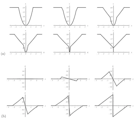
(2) 80. (a). (b) Figure 1: Layer thickness \eta(a) , and velocity u(b) evolution for the Airy model when the initial surface has a dry (contact) point and zero initial velocities. The parameters are Q=2, \gamma_{0}=1, \mu_{0}=0 , yielding a collapse time t_{c}=t_{s}\simeq 0.7854 . Time snapshots t=0,0.01,0.46,0.57,0.71,0.78.. It can be shown that the points. |x|=\sqrt{Q}/\gamma_{0} ,. where the parabola joins the constant background, each split. and evolve along distinct curves in the (x, t) ‐plane, which are among the characteristics of system (1.1), i.e., solutions of the ODE’s. \dot{x}\pm=\lambda\pm\equiv u(x\pm(t), t)\pm\sqrt{\eta(x\pm(t),t)}. (1.4). where the quantities (Riemann invariants) (1.5). R_{\pm}=u\pm 2\sqrt{\eta}. maintain their initial values. These curves emanating from the junction points bracket simple waves of sys‐. tem (1.1), that is, solutions for which \eta and u are functionally related. In the half domain x\geq 0 such simple wave solution, \eta\equiv N(x, t) and u\equiv V(x, t) say, can be expressed in closed form, albeit implicitly, through an auxiliary variable \sigma_{0}(x, t)\in[1, \infty ):. N(x, t)=\sigma_{0}Q(\sqrt{\sigma_{0}}-\sqrt{\sigma_{0}-1})^{2} , V(x, t)=2\sqrt {N(x,t)}-2\sqrt{Q} . Here. \sigma_{0}. as a function of. x. and. t. (1.6). is defined by the solution of. x= \Lambda(\sigma_{0})(t-\frac{\sqrt{\sigma_{0}-1}+\sigma_{0} \arctan(\sqrt{\sigma_{0}-1}) {2\sigma_{0}\sqrt{\gam a_{0} )+ \frac{\sqrt{Q\sigma_{0} -\sqrt{Q(\sigma_{0}-1)} {\sigma_{0}\sqrt{\gam a_{0}. ,. (1.7).

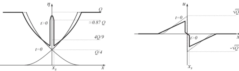
(3) 81 81 where we have used the shorthand notation. \Lambda. for the characteristic velocity \lambda_{-},. \Lambda(\sigma_{0})=3\sqrt{Q}\sigma_{0}(1-\sqrt{1-\frac{1}{\sigma_{0} - \frac{2}{3\sigma_{0} ). ,. (1.8). for any given point (x, t) in the spatio‐temporal half‐plane x>0 and t>0 . Symmetric and antisymmtric extensions, respectively for \eta and u , when x<0 complete the exact solution form. A typical evolution of the initial data according of the exact solution constructed piecewise with the above results is depicted in figure 1. As seen from the last panel in the figure, the solution develops a singularity in finite time, corresponding to \gamma(t)arrow\infty , i.e., the parabolic core of the piecewise solution collapses onto a vertical segment of length. Q/4 . From the solution of the ODE’s (1.3), and/or from the implicit expressions of the bracketing simple waves (1.7), (1.6) by finding the first time at which the partial derivative N_{x} becomes infinite, it can be shown that this verticality at the origin, or “global gradient catastrophe” (as the derivative of \eta and u become infinite not just at single points but for all points in an interval of the range of \eta(x, \cdot) , occurs at the time. t=t_{c} \equiv\frac{\pi}{4\sqrt{\gamma_{0}. (1.9). Evolution beyond the gradient catastrophe. As seen in the last panel of figure 1(a), the singularity of the dependent variables (\eta, u) at the time. t=t_{c}. is. that of a jump discontinuity for both fields. The segment connecting the free surface to the bottom at x=0 represents colliding water masses at that point and time, and it is natural to remove it to obtain a connected. domain for the water layer at times t=t_{c}^{+} . However, the discontinuity from the values \sqrt{Q} (left) to -\sqrt{Q} (right) in the velocity u would remain at x=0 , and it is natural to expect that this jump would result in. the instantaneous rising of the fluid in a neighbourhood of this location. This can be determined precisely. by studying the initial value problem for system (1.1) corresponding to initial data obtained by the “wings” solutions N(x, t_{c}) and V(x, t_{c}) in (1.6), appropriately reflected across the origin. Looking at the limit xarrow 0^{+} of N(x, t_{c}) , it can be seen that this function is not differentiable at the origin; more precisely. N(x, t_{c}) \sim\frac{Q}{4}+\frac{3^{2/3}\gamma_{0}^{1/3}Q^{2/3} {8}x^{2/3}+ o(x^{2/3}). as. xarrow 0. .. (1.10). The consequences of this branch point singularity on the evolution of the “new” initial data after gradient catastrophe are mostly of technical nature, and it is worth studying a class of data that removes the fractional power obstacle, yet captures the main features of the time advancement past the t=t_{c}. and. Consider the initial data obtained by splicing together two “Stoker” simple waves (see [1]) crossing at \eta(0,0)=\eta_{0},. N_{S}(x,t)=\{begin{ary}l Q,\frac{1}9(\frac{x-_d}{t+_c}2\sqrt{Q})^2, \frac{1}9(-\frac{x+_d}{t+_c}2\sqrt{Q})^2, Q \end{ary} V_{S}(x,t)=\{beginary}{l 0,x\geq_{Q} \frac{2}3\frac{x-_d}{t+_c}-\fra{2}3\sqrt{Q},0<x _{Q} \frac{2}3\frac{x+_d}{t+_c}\fra{2}3\sqrt{Q},-x_ < 0 ,x\leq-_{Q} \end{ary}. x=0. (1.11). With. x_{d}= \frac{1}{4}\sqrt{\frac{3Q}{g_{0} , t_{c}=\frac{1}{2}\sqrt{\frac{3} {g_{0} , x_{Q}=\sqrt{Q}t+\frac{3}{4}\sqrt{\frac{3Q}{g_{0}. .. (1.12). one can obtain a configuration that closely resembles that of the pair N(x, t_{c}), V(x, t_{c}) in (1.6) sketeched in figure 2, dashed curves. As depicted in this figure, the evolution out of these initial data for times. t>0.

(4) 82. Figure 2: Schematics of the initial condition (dash) and evolution (solid) with shock development at short times t>t_{c} for the Airy solutions (1.11). The thin segments of parabolae are removed from the initial data and the shocks develops from the initial discontinuity in the velocity (right panel). (corresponding to times t>t_{c} for the original case of (1.2)) involves the generation of two symmetrically placed shocks in both the \eta and u fields, moving away from the origin, with an intermediate region between the shock corresponding to fluid slowly filling the initial time “hole” at x=0, \eta=Q/4 . These shocks move. over the background given by the evolution of the Stoker waves (1.11) for t>0. Let x_{s}(t) be the position of the right‐going shock. We introduce the “unfolding” coordinates (\xi, \tau) to set the shock positions at fixed locations in time, e.g., \xi=\pm 1 , which can be achieved by. \xi\equiv\frac{x}{x_{s}(t)}) \tau\equiv\log(x_{s}(t) ,. (1.13). so that the Jacobian of this transformation reads. \partial_{x}=\frac{1}{x_{s} \partial_{\xi}, \partial_{t}=\frac{\dot{x}_{s} {x_ {s} (\partial_{\tau}-\xi\partial_{\xi}). (1.14). With this mapping, the Airy’s system (1.1) assumes the form (with a little abuse of notation by maintaining the same symbols for dependent variables). \frac{\partial\eta}{\partial\tau}-\xi\frac{\partial\eta}{\partial\xi}+\frac{1} {\dot{x}_{s} \frac{\partial}{\partial\xi}(\etau)=0,\frac{\partialu} {\partial\tau}-\xi\frac{\partialu}{\partial\xi}+\frac{1}{\dot{x}_{s} \frac{\partial}{\partial\xi}(\frac{u^{2} {2}+\eta)=0 .. (1.15). Here \dot{x}_{s} is a placeholder for the expression that couples the evolution equation for the physical time t to the new evolution variable \tau . The shock position evolves according to the equation that defines \dot{x}_{s} in terms of the jump amplitudes [\eta] and [\eta u] :. \frac{d(e^{\tau})}{dt}=\dot{x}_{s}=\frac{[\eta u]}{[\eta]}=\frac{N(x_{s}(t),t) V(x_{s}(t),t)-\eta(1,\tau(t) u(1,\tau(t) }{N(x_{s}(t),t)-\eta(1,\tau(t) }, x_{s} (0)=0 ,. (1.16). so that, in the new variables,. \frac{dt}{d\tau}=\frac{e^{\tau}(N(e^{\tau},t(\tau) -\eta(1,\tau) }{N(e^{\tau}) t(\tau) V(e^{\tau},t(\tau) -\eta(1,\tau)u(1,\tau)},. t(\tau)arrow 0. as. \tauarrow-\infty. .. (1.17). Here and in the following, we have suppressed the subscript s for the Stoker simple‐waves, and adopted the usual square‐bracket notation for jumps defined as the difference between values .\pm at the right and left of. the shock location, respectively (see e.g., [2]). From these expressions, the system governing the evolution of the “inner” solution between shocks consists of this ordinary differential equation together with the partial.

(5) 83 differential equations (1.15), to be solved within the strip \xi\in[0,1] (by symmetry only half the \xi domain [−1, 1] may be used) subject to the boundary conditions. u(0, \tau)=0, u(1, \tau)=V(e^{\tau}, t(\tau) +\sqrt{\frac{(N(e^{\tau},t(\tau) - \eta(1,\tau) ^{2}(N(e^{\tau},t(\tau) +\eta(1,\tau) }{2N(e^{\tau},t(\tau) \eta(1, \tau)}. .. (1.18). The first equality is a consequence of the antisymmetry of the velocity, u(\xi, \tau)=-u(-\xi, \tau) . The second relation expresses, in terms of the new independent variables, the consistency condition for the shock speed. \dot{x}_{s}=\frac{[\eta u^{2}+\eta^{2}/2]}{[\eta u]} ,. (1.19). [u]^{2}= \frac{[\eta]^{2}(\eta_{+}+\eta_{-}) {2\eta+\eta_{-} ). (1.20). which can be manipulated to. whence the second relation in (1.18) follows. The boundary‐value problem (1.18) for the evolution equations (1.15) and (1.17), by depending on the unknown \eta at the boundary, \eta(1, \tau) , is reminiscent in its structure of the classical (irrotational) water‐wave problem, wherein the unknowns, the free surface location and the velocity potential along it, determine and in. turn are determined by the solution of a PDE (for water wave problem, the Laplace equation for the velocity potential in the fluid domain). Just as in that case, an additional equation has to be provided at the boundary, which has its analog in (1.17). Similarly to the water‐wave problem, the resulting structure is highly nonlinear and hence hardly amenable to closed form solutions. To make progress, observe that the “initial” data as \tauarrow-\infty , i.e., t=0 , are given by u(\xi, -\infty)=0 and \eta(\xi, -\infty)=Q^{*} , where Q^{*} is the constant solution of the cubic equation. -2\sqrt{Q}+2\sqrt{N(0,0)}+\sqrt{\frac{(N(0,0)-Q^{*})^{2}(N(0,0)+Q^{*})}{2N(0,0) Q^{*} }=0. ,. (1.21). subject to the condition Q^{*}>N(0,0) . Thus, the initial time evolution can be followed by the linearization of system (1.15)-(1.17) around \eta=Q^{*} and u=0 . This approach is mostly straightforward, though the details. are bit involved, and will be reported elsewhere. Suffices to say that the initial evolution as. \tauarrow-\infty. (and so. tarrow 0^{+}) is asymptotic to. \eta(\xi, \tau)=Q^{*}+\frac{1}{2}(F(e^{\tau}\xi-\Phi(\tau))+F(-e^{\tau}\xi- \Phi(\tau)) ,. u( \xi, \tau)=\frac{1}{2\sqrt{Q^{*} }(F(e^{\tau}\xi-\Phi(\tau))-F(-e^{\tau}\xi- \Phi(\tau)) , (1.22). for any function F(\cdot) of sufficient regularity, with the function. \Phi. defined by. \Phi(\tau)\equiv\sqrt{Q^{*} \int_{-\infty}^{\tau}e^{\tau'}\phi_{0}(\tau') d\tau' ,. (1.23). \phi_{0}(\tau)=\frac{N(e^{\tau},t(\tau) -Q^{*} {N(e^{\tau},t(\tau) V(e^{\tau}, t(\tau) }. (1.24). where the integrand \phi_{0}(\tau) is. Here. s_{0}. is the initial shock speed \dot{x}_{s} at t=0^{+} , and the initial conditions on the system’s solution (\eta, u) as require F(0)=0 . Substitution of these expressions evaluated at \xi=1 into the linearized version of. \tauarrow-\infty. the boundary condition (1.18) leads to a functional equation for F , coupled to the evolution (linearized) equa‐ tion (1.17) for t(\tau) . By assuming sufficient regularity for F , the functional equation can be solved approximately by Taylor series. The result to second order is. \eta(\xi, \tau)\sim Q^{*}-F'(0)\Phi_{0}e^{\tau}+(-F'(0)\Phi_{1}+\frac{1}{2} F"(0)(\xi^{2}+\Phi_{0}^{2}) e^{2\tau} ,. u( \xi, \tau)\sim\frac{F'(0)}{\sqrt{Q^{*} \xi e^{\tau}-\frac{F"(0)} {\sqrt{Q^{*} \Phi_{0}\xi e^{2\tau}. ,. (1.25) (1.26).

(6) 84 where the Taylor coefficients F'(0), F"(0) and those for the asymptotic expansion of \Phi(\tau)\sim\Phi_{0}e^{\tau}+\Phi_{1}e^{2\tau} are, respectively,. F'(0)\simeq-0.22215\sqrt{g_{0}Q}, F"(0)\simeq-0.58487g_{0} ,. (1.27). and. \Phi_{0}=\frac{\sqrt{Q^{*} (4Q^{*}-Q)}{Q^{3/2} \simeq 2.33087, \Phi_{1}= \sqrt{g_{0}Q^{*} (Q+4Q^{*})^{2}3\sqrt{3}Q^{3}\simeq-3.6325\sqrt{\frac{g_{0} {Q}. ,. with the parametrization (1.12) for the initial data. The asympotics for the shock location computed as. (1.28) x_{s}. is similarly. \tauarrow-\infty.. Returning to the original physical variables \eta(x, t), u(x, t) , the asymptotic expressions (1.25),(1.26) lead to. \eta(x, t)\sim Q^{*}-F'(0)\Phi_{0}s_{0}t-(F'(0)\Phi_{0}s_{1}+(F'(0)\Phi_{1}- \frac{1}{2}F"(0)\Phi_{0}^{2})s_{0}^{2})t^{2}+\frac{1}{2}F"(0)x^{2} ,. u(x, t) \sim\frac{x}{\sqrt{Q^{*} }(F'(0)-F"(0)\Phi_{0}(s_{0}t+s_{1}t^{2}) , x_{s}(t)\sim s_{0}t+s_{1}t^{2} ,. with. s_{0}\simeq 0.400969\sqrt{Q} ,. (1.29) (1.30). sı \simeq 0.11703\sqrt{g_{0}Q} ,. (1.31). as tarrow 0^{+} . Note that the asymptotic validity of these expressions is established within the unfolding variable. formulation, and hence it is not necessarily maintained after the mapping (1.13), unless this is also consistently expanded with the asymptotics. Nonetheless, the above expression for the \eta and u field reveal that the layer thickness \eta jumps, at time t=0^{+} , to about 87% of the background rest thickness Q , and grows linearly in time while maintaining a local parabolic shape, fixed in time at this order. Similarly, the local velocity u jumps from a discontinuity of amphtude 2\sqrt{Q} at x=0 to a continuous linear profile between shocks, with negative slope which evolves linearly in time. Of course, further progress is most easily achieved by resorting to numerical methods. However, we remark that standard WENO algorithms we have implemented are not able to capture the above details at short times, and one has to resort to the unfolding variable system which can be integrated numerically with spectrally accurate codes. These, once validated on the analytical results, can provide information on the time evolution. well past the initial times. Numerical tools are even more challenged by the full case of initial data (1.2) when going beyond the gradient catastrophe, since this case poses additional difficulties due to the singular behavior of N(x, t_{c}) at the origin. The main details of this and other cases will be reported elsewhere. Acknowledgments. This isjoint work with Gregorio Falqui (Universitá of Milano‐Bicocca), Giovanni Ortenzi (Universitá of Milano‐ Bicocca), Marco Pedroni (Universitá di Bergamo), and Giuseppe Pitton (Imperial College London), and is largely based on a paper by these authors which is being submitted for publication. The author thanks the hospitality of the ICERM’s program “Singularities and Waves in Incompressible Fluids” in the Spring of 2017, the support by the National Science Foundation under grants RTG DMS‐0943851, CMG ARC‐1025523, DMS‐1009750, DMS‐1517879, and by the Office of Naval Research under grants N00014‐18‐1‐2490 and DURIP N00014‐12‐1‐0749. All investigators gratefully acknowledge the auspices of the GNFM Section of INdAM under which part of this work was carried out, and the Dipartimento di Matematica e Applicazioni of Univer‐ sità Milano‐Bicocca for its hospitality; travel support by grant H2020‐MSCA‐RISE‐2017 Project No. 778010 IPaDEGAN is also acknowledged. Last, but not least, the author wishes to thank the organizers for inviting him to the Workshop on Nonlinnear Water Waves held in Kyoto, May 22ns to 26th, in honor of Professor Mitsuhiro Tanaka on the occasion of his retirement.. References. [1] Stoker, J.J. (1957) Water Waves: The Mathematical Theory with Application\mathcal{S} . Wiley‐Interscience, New York, NY.. [2] Whitham, G.B. (1999) Linear and Nonlinear Waves. Wiley, New York, NY..

(7)