Turbulence in quantum hydrodynamics (Mathematical Analysis of Viscous Incompressible Fluid)

全文

(1)148. 数理解析研究所講究録第2058巻 2017年 148-161. Turbulence in quantum. hydrodynamics. Michikazu Kobayashi Department Physics, Kyoto University. By numerically solving the Gross‐Piteavskii equation with the energy injec‐ dissipation, we study quantum turbulence comprised of quantized vortices with discrete circulations. We consider two opposite cases of fully developed quantum turbulence with strong energy injections and transi‐ tion and. tion from quantum turbulence with vortices to vortex‐free state with weak energy injections. With strong energy injections, the obtained energy spec‐ trum for fully developed quantum turbulence has two scaling regions sepa‐. rated the. by the scale. mean. of the. inter‐vortex. mean. inter‐vortex distance. In scales. distance, the. larger than. energy spectrum shows the well‐known. Kolmogorov law with the exponent −5/3. In scales smaller than the mean distance, on the other hands, the exponent of the energy spec‐ trum changes to −7/5 suggesting that quantum turbulence is dominated by the Kelvin‐wave cascade process of a single vortex line. With weak energy injections, the vortex‐line density monotonically decreases with de‐ creasing the strength of the energy injection and vanishes at the certain value of the energy injection. Close to the transition point, the vortex‐line density can be regarded as the order parameter of the transition, showing its power‐law behavior with the critical exponent 0.81. This value of the inter‐vortex. critical exponent is consistent with that for the. (3 + 1)‐dimensional directed. percolation, which suggests the same underlying physics of the directed percolation and quantum turbulence.. 1. for two transitions. Introduction. Quantum fluid realized. in. supefluid helium. and atomic Bose‐Einstein condensates. near. the absolute. temperature has become one great topic in various field of physics such as low temperature physics, fluid physics, quantum physics, statistical physics, cosmology, and so on [1]. The most important hydrodynamic property of quantum fluid is that any kind of flow is either inviscid and zero. irrotational. or carried by quantized vortices with a fixed circulation. The above feature of quantum originates from the spontaneous breaking of the U(1) symmetry for the phase shift of the order parameter and the flow is given as the gradient of the phase of the order parameter. Quantized vortices in quantum fluid are realized as topological line defects as a result of the U(1) symmetry breaking. Under the mean‐field approximatlon and assuming the short‐ranged inter‐particle interaction, we can write down the equation for the time evolution of the order parameter known as the Gross‐ Pitaevskii (GP) equation which has the form of the Non‐linear Schrödinger equation having the third order nonliearity. The GP equation satisfies the hydrodynamic property of quantum fluid and enables us to study the quantum hydrodynamics. One of the most active topics in the quantum hydrodynamics is quantum turbulence realized in quantum fluid. As well as conventional turbulence with a large number of eddies having various. fluid.

(2) 149. scales described. by the Navier‐Stokes equation, quantum turbulence is realized as temporary and spatially complicated structures of quantized vortices. The important differences between quan‐ tized vortices in quantum turbulence and eddies in conventional turbulence are (i) circulations of quantized vortices are concentrated in their cores and (ii) possible circulations are discrete. In this. work,. we. numerically study the GP equation. and consider two. topics of quantum turbulence. in. which the above characteristics of quantum vortices plays an important role: (i) the kinetic energy spectrum of the statistically steady state of fully developed quantum turbulence and (ii) transition. from turbulent to vortex‐free states. This. proceeding is organized as follows. In Sec. 2, we briefly show how to derive the GP equation microscopic many‐body Schrödinger equation with the mean‐field approximation and the short‐ranged inter‐particle interaction potential [2]. The fundamental hydrodynamic property of the GP equation is also reviewed. In Secs. 3 and 4, we show our results about the energy spectrum of fully developed quantum turbulence (in Sec. 3) and transition from turbulent to vortex‐free states (in Sec. 4). Section 5 provides the summary and concluding remarks. from the. GP. 2 2.1. equation and quantum hydrodynamics. Bose‐Einstein condensation and GP. We start from the. equation. many‐Uody Schrödinger equation. with N ‐particle bosons with the. mass. M in. 3‐dimensional space:. i\displaystyle\hslash\frac{\partial}{\partialt}$\Psi$(x_{1},\cdots,x_{N},t)=\{-\sum_{i=1}^{N}\frac{\hslash^{2} {2M}$\Delta$_{i}+\frac{1}{2}\sum_{i\neqj}V(x_{i}-x_{j})\}$\Psi$(x_{1},\cdots,x_{N},t) \equiv H_{N} $\Psi$ (x_{1}, \cdots x_{N}, t). where $\Psi$ (x_{1}, \cdots , x_{N}) is the N ‐particle. wave. function. ,. satisfying. $\Psi$ (x_{1}, \cdots X_{i}, \cdots x_{j}, \cdots x_{N})= $\Psi$(x_{1}, \cdots x_{j}, \cdots x_{i}, \cdots x_{N}) for bosons.. V(x_{i}-x_{j}). (1). (2). ,. is the. two‐Uody inter‐particle interaction potential. In this proceeding, we 1‐body potential such as a harmonic trap, magnetic and electric fields. following density matrix:. do not consider the external We define the. $\rho$^{(2)}(x, y, t)\displaystyle \equiv\int d^{3}x_{2} \int d^{3}x_{N}$\Psi$^{*}(x, x_{2}, \cdots , x_{N}, t) $\Psi$(y, x_{2}, \cdots , x_{N}, t) With. taking y\rightarrow x , the density matrix sometimes encounter the condition. gives the density $\rho$(x, t). .. In the limit of. $\rho$^{(2)}(x,y, t)\rightarrow$\psi$^{*}(x, t) $\psi$(y, t)\neq 0|x-y|\infty Eq. (4) is satisfied for the time‐independent ground eigenenergy E_{\mathrm{G} of the Hamiltonian H_{N} defined as If. state. |x-y|. (3) \rightarrow\infty , we. (4). .. $\Psi$_{\mathrm{G}0} for Eq.. E_{\mathrm{G} $\Psi$ Go (x_{1}, \cdots x_{N})=H_{N}$\Psi$_{\mathrm{G}0}(x\mathrm{i}, \cdots , x_{N}). .. ,. $\Psi$_{\mathrm{G}} (x_{1}, \cdots x_{N}, t)=e^{-iE_{\mathrm{G}}/\hslash}$\Psi$_{\mathrm{G}0}(x_{1}, \cdots x_{N}). (1). with the lowest. (5) ,.

(3) 150. then, the system. is defined. as. the Bose‐Einstein condensation state. Equation. (4). shows the spon‐ The. breaking of the U(1) symmetry for the global phase shift of the order parameter $\psi$(x) condensate density is defined as $\rho$_{\mathrm{c} \displaystyle \equiv| $\psi$|^{2}=|\lim_{|x-y|\rightar ow\infty}$\rho$^{(2)}| The condensate fraction taneous. .. .. |\displaystyle \lim_{|x-y|\rightarrow\infty}$\rho$^{(2)}(x, y)|. $\rho$_{\mathrm{c}. n_{\mathrm{c} \equiv\overline{ $\rho$}=\overline{\lim_{|x-y|\rightar ow 0}$\rho$^{(2)}(x,y)}. \{. \sim 0.1 ,. liquid 4He below. \sim>0.9. ultra‐cold atomic gas,. ,. 1. \mathrm{m}\mathrm{K},. (6). intensity of the symmetry breaking. The exact definition of the Bose‐Einstein conden‐ time‐dependent state has not been constructed yet, we here regard the time‐dependent Bose‐Einstein condensation state when Eq. (4) is satisfied for the time‐dependent wave function $\Psi$ measures. the. sation for the. [3]. We next consider the. following. mean‐field approximation:. $\Psi$ (x_{1}, \displaystyle \cdots x_{N}, t)\ap rox\prod_{i=1}^{N} $\psi$(x_{i}, t). (7). .. Equation (7) consists of two kinds of approximations. The first one is that $\Psi$ is approximated to be separated into single‐particle state, and the second one is all separated single‐particle state join the same state $\psi$(x, t) This approximation is rigorously satisfied only in the time‐independent ground state for the ideal Bose gas with V(x_{i}-x_{j})=0 for arbitrary pairs of i and j The approximation 1 in Eq. (7) gives the perfect Bose‐Einstein condensation with the unit condensate fraction n_{\mathrm{c} (6), and the single‐particle wave function $\psi$ in Eq. (7) just becomes the order parameter defined in Eq. (4). The necessary condition for the validity of the mean‐field approximation (7) is, therefore, that the condensate fraction n_{\mathrm{c} has to be close to unity. The density (or condensate density) is given by $\rho$(x, t)=| $\psi$(x, t)|^{2}. Inserting Eq. (7) into the Schrödinger equation (1), we obtain the non‐local GP equation .. .. =. i\displaystyle \hslash\frac{\partial}{\partial t} $\psi$(x, t)= \{-\frac{\hslash^{2} {2M} $\Delta$+\int d^{3}yV(x-y)| $\psi$(y, t)|^{2}\} $\psi$(x, t) where. we. rewrite. \sqrt{N-1} $\psi$(x, t). potential V(x-y). as. the. as. $\psi$(x, t). short‐ranged. .. We here. replace. the. ,. two‐Uody inter‐particle. (8) interaction. delta‐functional form. V(x-y)\displaystyle \approx\frac{4 $\pi$\hslash^{2}a_{s} {M} $\delta$(x-y)\equiv g $\delta$(x-y). .. (9). This assumption is valid when V(r) rapidly goes to zero for r\gg r_{0} with the effective length r_{0} , the $\rho$ is very low satisfying $\rho$ r_{0}^{3}\l 1 , and inter‐particle scattering energy is so low that almost. density. all inter‐particle scattering are s‐wave. The coefficient approximation, and a_{s} is the s‐wave scattering length. positive a_{s} We shortly note that the the approximation (9) gives .. 4_{\mathrm{T}}h^{2}a_{s}/M. [4].. be obtained within the Born. proceeding, we only consider the analysis of the many‐body Schrödinger equation (1) under. 1-n_{\mathrm{c} =\mathcal{O}(\sqrt{ $\rho$ a_{s}^{3} ). (10). ,. time‐independent ground state [5]. We therefore obtain the second necessary condition for validity of the mean‐field approximation (7) as $\rho$ a_{s}^{3} \ll 1 Inserting Eq. (9) into Eq. (8), we. for the the. can. In this. ..

(4) 151. finally. obtain the GP. equation. i\displaystyle \hslash\frac{\partial}{\partial t} $\psi$(x, t)=\{-\frac{\hslash^{2} {2M} $\Delta$+g| $\psi$(x, t)|^{2}\} $\psi$(x, t) In the. (11). .. following, we omit notations of the spatial and temporal dependence (x, t) equation (11) can be obtained from the following Hamilton equation:. for all functions.. The GP. ih\displaystyle\frac{\partial$\psi$}{\partialt}=\frac{$\delta$\mathcal{E} {$\delta\psi$^{*} ,\mathcal{E}=\intd^{3}x(\frac{\hslash^{2} {2M}|\nabla$\psi$|^{2}+\frac{g}{2}$\rho$^{2}). (12). ,. with the energy \mathcal{E} We here introduce the Lagrange multiplier to satisfy that the uniform state with the density $\rho$=$\rho$_{0} can be obtained by minimizing the energy as .. \displaystyle \mathcal{E}-g$\rho$_{0}\mathcal{N}\equiv \mathcal{E}-g$\rho$_{0}\int d^{3}x $\rho$\rightar ow \mathcal{E}=\int d^{3_{X} \{\frac{\hslash^{2} {2M}|\nabla $\psi$|^{2}+\frac{g}{2}( $\rho-\rho$_{0})^{2}-g$\rho$_{0}^{2}\} The. .. ground. (13). resulting GP equation becomes. i\displaystyle\hslash\frac{\partial$\psi$}{\partialt}=\{-\frac{\hslash^{2} {2M}$\Delta$+g($\rho-\rho$_{0})\}$\psi$ Eqs. (11) Eq. (11).. There is. difference between. the. $\psi$\rightar ow e^{-ig $\rho$ 0t/\hslash} $\psi$. no qualitative phase shift of $\psi$ as. 2.2. Hydrodynamic property. The time evolution of the. density. in. of GP. (14). and. where. v. is defined. as v. =. because. Eq. (14). can. be obtained. by. equation. $\rho$ becomes. \displaystyle\frac{\partial$\rho$}{\partialt}=-\nabla\cdot($\rho$v) velocity, and. (14). .. (\hslash/M)\nabla\arg[ $\psi$]. .. From this. (15). ,. equation,. v. can. be. regarded. as. the fluid. its time evolution is. \displaystyle\frac{\partialv}{\partialt}+\frac{1}{2}\nablav^{2}=-\frac{1}{M$\rho$}\nabla(\frac{g$\rho$^{2}{2})+\frac{\hslash^{2}{2M^{2}\nabla(\frac{$\Delta$\sqrt{$\rho$}{\sqrt{$\rho$}). (16). .. Equation (16) is the conventional Euler equation for the barotropic fluid with the pressure g$\rho$^{2}/2, we ignore the second term of the right‐hand side. This additional term which is absent from the Euler equation is known as the quantum pressure. The energy \mathcal{E} in Eq. (13) is rewritten as when. \displaystyle \mathcal{E}=\int d^{3_{X} \{\frac{M}{2} $\rho$ v^{2}+\frac{g}{2}( $\rho-\rho$_{0})^{2}-g$\rho$_{0}^{2}+\frac{\hslash^{2} {2M}|\nabla\sqrt{ $\rho$}|^{2}\} The first three terms. are. (17). .. conventional fluid energy and the last term is defined. as. the quantum. originated from the quantum pressure in Eq. (16). The outstanding difference between quantum hydrodynamics and classical one is that the fluid velocity v is irrotational everywhere except for the one‐dimensional singular lines of the order parameter $\psi$ The order parameter $\psi$ rapidly decreases in the scale of the healing length $\xi$ \hslash/\sqrt{Mg$\rho$_{0}} close to the lines and vanishes on the lines, and the phase \arg[ $\psi$] changes by integer energy. .. =.

(5) 152. multiple. of 2 $\pi$ around the lines.. circulation for. a. closed. loop. These. singular lines. are. known. quantized vortices, and the. as. \mathcal{L} becomes. \displaystyle \oint_{\mathcal{L} dl\cdot v=\frac{hn}{M}, n\in \mathb {Z}. quantized vortices pierce the loop \mathcal{L} the integer n takes nonzero values as n\neq 0 Equa‐ that all rotational flow are carried by quantized vortices with discrete circulation implies (18) hn/M If we omit the quantum pressure term in Eq. (16), the quantum nature in hydrodynamics with discretized circulations disappears. Only. when. (18). .. .. ,. tion. .. Generating statistically steady. 2.3. turbulent state. conserves not only total number of particles \mathcal{N} but also the energy statistically steady and non‐equiliUrium turbulent state because it has neither the energy injection in large scales nor the energy sink in small scales. We therefore modify the GP equation (14) to obtain statistically steady turbulence.. The. original. GP. equation (14). \mathcal{E} , and cannot create. 2.3.1. Energy. We consider the. sink in GP. equation. Ginzburg‐Landau (GL) equation. \displaystyle \hslash\frac{\partial}{\partial t} $\psi$=- $\gam a$\{-\frac{\hslash^{2} {2M}\triangle+g( $\rho-\rho$_{0})\} $\psi$ Although this equation is similar particles \mathcal{N} nor the energy \dot{\mathcal{E} and. to the GP. equation, it. (19). .. neither the total number of. conserves. $\psi$ is attracted into the uniform ground state $\rho$(x, t\rightarrow\infty)\rightarrow$\rho$_{0} under the time evolution with losing the energy \mathcal{E} Here $\gamma$>0 is the dissipation constant. We combine the GP equation (14) and the GL equation (19) as ,. the. wave. function. .. \displaystyle \hslash\frac{\partial}{\partial t} $\psi$=-(i+ $\gamma$)\{-\frac{\hslash^{2} {2M} $\Delta$+g( $\rho-\rho$_{0})\} $\psi$ As well. as. rewritten. the GL equation,. $\psi$. is attracted in the uniform. ground. (20). .. state.. This. equation. can. be. as. \displaystyle\frac{\partial$\rho$}{\partialt}+\nabla\cdot($\rho$v)=\frac{2$\gam a$}{\hslash}\{ frac{\hslash^{2} {2M}\sqrt{$\rho$}\triangle\sqrt{$\rho$}-\frac{M}{2}$\rho$v^{2}-g$\rho$($\rho-\rho$_{0})\} \displaystyle\frac{\partialv}{\partialt}+\frac{1}{2}\nablav^{2}=-\frac{1}{$\rho$}\nabla(\frac{g$\rho$^{2}{2M})+\frac{\hslash^{2}{2M^{2}\nabla(\frac{$\Delta$\sqrt{$\rho$}{\sqrt{$\rho$})+\frac{$\gam a$\hslash}{2M}\nabla\{ frac{\nabla\cdot($\rho$v)}{$\rho$}\. (21a). ,. .. (21b). right‐hand side of Eq. (21b) works as the diffusion with the effective kinematic $\gamma$\hslash/(2M) Equation (21a) shows that the total number of particles \mathcal{N} is not To avoid this, we introduce the time dependence of $\rho$_{0} as $\rho$_{0}=$\rho$_{0}(t) to satisfy. The last term of the. viscosity. $\nu$_{\mathrm{e}\mathrm{f}\mathrm{f}. \equiv. conserved either.. .. \displaystyle \int d^{3}x \{\frac{\hslash^{2} {2M}\sqrt{ $\rho$}\triangle\sqrt{ $\rho$}-\frac{M}{2} $\rho$ v^{2}-g $\rho$( $\rho-\rho$_{0})\}=0. .. (22). Introducing the dissipation term $\gamma$ can be phenomenologically understood as the interaction between the condensate and its fluctuations by the thermal environment and the discrepancy from the mean‐ field approximation..

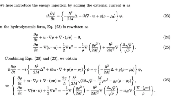
(6) 153. Energy injection. 2.4. in GP. We here introduce the energy. equation. injection by adding the external. current. i\displaystyle \hslash\frac{\partial $\psi$}{\partial t}=\{-\frac{\hslash^{2} {2M} $\Delta$+ih\nabla\cdot u+g(p-$\rho$_{0})\} $\psi$ In the. hydrodynamic form, Eq. (23). is rewritten. \displaystyle \frac{\partial $\rho$}{\partial t}+u\cdot\nabla $\rho$+\nabla\cdot( $\rho$ v)=0. u as. (23). .. as. (24). ,. \displaystyle\frac{\partialv}{\partialt}-\nabla(v\cdotu)+\frac{1}{2}\nablav^{2}=-\frac{1}{$\rho$}\nabla(\frac{g$\rho$^{2} {2M})+\frac{\hslash^{2} {2M^{2} \nabla(\frac{\triangle\sqrt{$\rho$} {\sqrt{$\rho$} ) Combining Eqs. (20). and. (23),. we. (25). .. obtain. \displaystyle \hslash\frac{\partial $\psi$}{\partial t}=-i\{-\frac{h^{2} {2M}$\Delta$^{2}+ihu\cdot\cdot\nabla+g( $\rho-\rho$_{0})\} $\psi$- $\gamma$\{-\frac{\hslash^{2} {2M} $\Delta$+g( $\rho-\rho$_{0})\} $\psi$, \Leftrightar ow. \left{bgin{ary}l \frac{prtial$\ho}{\partil}+u\cdotnabl$\rho+nabl\cdot($\rhov)=\frac{2$\gam $}{\hsla }\{frac\hsl ^{2} M\sqrt{$\ho}$\Delta$\sqrt{p}-\fac{M}2$\rhov^{2}-g$\rho($\rho-p_{0})\,&(26)\ frac{\prtialv}{\partil}-\nabl(u\cdotv)\cdot+frac{1}2\nablv^{2}=-\frac{1}$\rho}nabl(\frac{g$\rho^{2} M)+\frac{hsl ^{2} M^{2}\nabl(\frac{$\Delta$\sqrt{$\ho}{\sqrt$\ho})+$\nu_{mathr{e}\mathr{f}\mathr{f}\nabl {\fracnbla\cdot($\rhov)}{$\rho}.& \end{ary}\ight.. Eq. (26) under the condition (22) for the conservation of the total number of particles injection and the sink, we can obtain the statistically steady and non‐ equilibrium state. We solve. \mathcal{N}. 3. .. With both the energy. Energy spectrum. Figure 1: dissipation In this. Wave‐number rate. of. fully developed quantum. dependence. of the energy spectrum. -2 $\nu$ k^{2}E_{v}(k) (dashed line).. turbulence. E_{v}(k) (solid line). and the energy‐. section, we report our result for the energy spectrum of fully developed quantum tur‐ by the numerical simulation of Eq. (26). Before discussing the energy spectrum. bulence obtained.

(7) 154. of quantum turbulence, we briefly review the energy spectrum of uniform, isotropic, and fully‐ developed classical turbulence obeying the incompressible Navier‐Stokes equation. Figure 1 shows an. outline of the. kinetic‐energy spectrum E_{v}(k). defined. as. E_{v}(k)=\displaystyle\frac{1}{L^{3} \int\frac{k^{2}d$\Omega$_{k} {(2$\pi$)^{3} \frac{1}{2}\langle|\tilde{v}|^{2}\rangle. (27). ,. where \overline{v} is the Fourier transformation of v, \displaystyle \int d$\Omega$_{k} is the solid‐angle integration in the wave‐number space at k |k| , and \{\cdots\} is the averaged over the time. There are only two scales l_{F} and l_{ $\nu$}. =. The scale. l_{F} is that of the. energy. injection and usually the. same. order. as. the system size L. .. The. scale l_{\mathrm{v} is that where the energy dissipation by the kinematic viscosity $\nu$ becomes dominant, i.e., the wave‐number dependent energy dissipation rate 2\mathrm{v}k^{2}E_{v}(k) becomes maximal at k\approx 1/l_{ $\nu$} The .. energy‐dissipating rate $\epsilon$ defined by. scale l_{ $\nu$} is determined. by. the kinematic. viscosity. $\epsilon$=2 $\nu$\displaystyle \int dk ^{2}E_{v}(k) and it two. E_{v}(k). 1/l_{F}. numbers. is believed to. and the total energy. as. the. k \ll. \ll. .. ,. E(k)\propto$\epsilon$^{2/3}k^{-5/3} independent of the kinematic viscosity. dissipation. (28). ,. Kolmogorov length scale l_{ $\nu$}\approx \sqrt[4]{$\nu$^{3} / $\epsilon$ 1/l_{ $\nu$} the viscosity has little effect take the Kolmogorovs power‐law form:. be estimated. can. wave. $\nu$. In the inertial range between the energy spectrum, and. on. (29). ,. \mathrm{v}.. We next report our numerical simulation of Eq. (26). The details of the simulation is as follows. We prepare a discretized periodic cubic box with 20483 grids. The spatial interval between two. grids is taken to be $\Delta$ x=0.5 $\xi$ and the system size then becomes L=2048 $\Delta$ x= 1024 $\xi$. dissipation constant is set to be $\gamma$=0.1 To effectively create a fully developed turbulent state with many vortices, the incompressible external current v is more suitable than the compressible nearest. ,. The. one.. u_{\mathrm{r}. .. The external current. u. is fixed. as. follows. We first create smoothed random external current. as. u_{\mathrm{r},i =\displaystyle \frac{u_{0} {8}\sum_{n_{x},n_{y},n_{z}=\pm 1}\cos(\frac{2 $\pi$ n\cdot x}{L}+$\theta$_{i,n}) for i. (30). ,. Here - $\pi$ < $\theta$_{i,n} \leq $\pi$ take uniformlỳ random values. The external current u_{\mathrm{r} is x, y, z gradually changing in a length scale of the system size L and can be decomposed into the com‐ pressible and incompressible parts. by the Helmholtz decomposition. We adopt the incompressible part of u_{\mathrm{r} as u We solve Eq. (26) with the pseudo‐spectral method in space and the fourth‐ordered Runge‐Kutta method in time. Here, we define the kinetic‐energy spectrum E_{v}(k) as =. .. ,. .. \displaystyle \int dkE_{v}(k)=\frac{1}{\mathcal{N} \int d^{3}x\frac{1}{2}\langle $\rho$ v^{2}\rangle \Leftrightar ow E_{v}(k)=\frac{1}{\mathcal{N} \int\frac{k^{2}d$\Omega$_{k} {(2 $\pi$)^{3} \frac{1}{2}\{|F[\sqrt{ $\rho$}v]|^{2}\rangle where a. F[A]. ,. (31). is the Fourier transformation of A.. Figure 2 show arbitrary initial. our. numerical results.. state such. as. a. After. a. uniform state. long time $\psi$ \sqrt{$\rho$_{0} =. ,. evolution of we. can. Eq.. obtain. a. (26) starting from statistically steady.

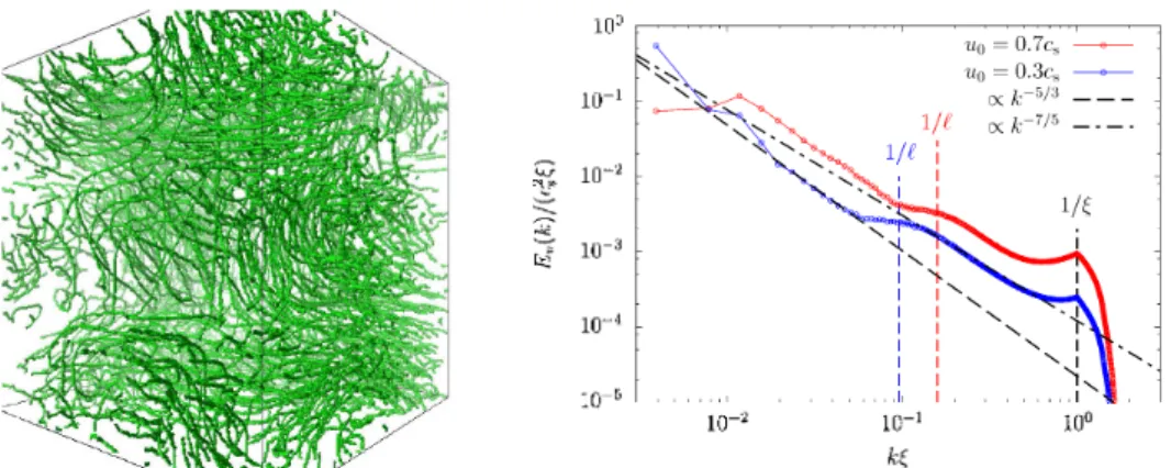
(8) 155. Figure 2: Left panel: Snapshot of a spatial vortex configuration for the statistically steady state of Eq. (26) with u_{0} 0.7c_{\mathrm{s} where c_{\mathrm{s} \equiv \sqrt{2g$\rho$_{0}}/M is the sound velocity. Right panel: Kinetic energy spectrum E_{v}(k) defined in Eq. (31) with the amplitude of the external current u_{0} =0.3c_{\mathrm{s}} 0.7c_{\mathrm{s} (red curve). Here, we take an ensemble average \{\cdots ) by taking the (blue curve) and u_{0} =. ,. =. mean over. 10 different external currents. external current. displayed. u. .. The. wave. for each v_{0} with the. u. with different. 1/\ell corresponding. number. corresponding. $\theta$_{i,j}. and. to the. over. mean. 1000 different times for each. inter‐vortex distance P is also. color.. independent of the initial states. The left panel shows one snapshot of a spatial vortex configuration. The right panel shows the obtained kinetic energy spectrum E_{v}(k) with different amplitudes of the external current u_{0} 0.3c_{\mathrm{s} and 0.7c_{\mathrm{s} In both cases, there are two power‐law regions E_{v}(k) \propto k^{-$\eta$_{1\mathrm{o}\mathrm{w} } .high separated by a bump structure, where two exponents $\eta$_{1\mathrm{o}\mathrm{w} ,high can be obtained by the fitting as $\eta$_{1\mathrm{o}\mathrm{w} 1.62(24) and $\eta$_{\mathrm{h}\mathrm{i}\mathrm{g}\mathrm{h} 1.42(15) for lower and higher k regions respectively. The exponent $\eta$_{1\mathrm{o}\mathrm{w} is very close to 5/3\simeq 1.67 and we expect that the Kolmogorov spectrum in Eq. (29) is also executed even in quantum turbulence and the quantum pressure in Eq. (16) has little effect on the property of quantum turbulence in large scales. This Kolmogorov‐like spectrum does not continue to high wave‐number region with the bump structure. The end of the Kolmogorov‐like spectrum might be considered to be determined by the dissipation such that the Kolmogorov spectrum in classical turbulence does not continue at k\approx 1/l_{ $\nu$} We here estimate the state. =. .. =. =. .. effective. \sqrt[4]{iJ_\mathrm{e}\mathrm{f}\mathrm{f}^{3}/$\epsilon$}. Kolmogorov length l_{ $\gamma$}\equiv Eq. (28) because. be estimated from. for. Eq. (26).. The total energy. dissipation. rate. $\epsilon$. cannot. the kinetic energy may not only be dissipated with $\gamma$ but also be transfered into the quantum energy defined in Eq. (17) through the quantum pressure. Instead of Eq. (28), we estimate the energy dissipation rate $\epsilon$. $\epsilon$\displaystyle\equiv-\langle\lim_{t\rightar ow0}\frac{\partial\mathcal{E} {\partialt}\ \simeq-\langle\frac{$\epsilon$(t=$\Delta$t)-$\epsilon$(t=0)}{$\Delta$t}\rangle after. (32). 0 at t= 0 We then estimate the effective suddenly switching off the external current u Kolmogorov length l_{ $\gamma$}\approx 0.8 $\xi$ and 0.5 $\xi$ for u_{0} =0.3c_{\mathrm{s}} and 0.7c_{\mathrm{s} respectively, and the wave‐number 1/l_{ $\gamma$} is much far from the position of the bump. We have also checked that the overall shape of E_{v}(k) at k < 1/ $\xi$ including the position of the bump and exponents $\eta$_{1\mathrm{o}\mathrm{w} ,high hardly change with the larger dissipation constant $\gamma$=0.3 Therefore, we can conclude that introducing the dissipation =. .. ..

(9) 156. constant $\gamma$ is not the. origin. of the end of the. Kolmogorov‐like spectrum. with the appearance of the. bump. As another candidate of the end of the. Kolmogorov‐like spectrum, we expect that the quantum negligible in this scale. Because the quantum pressure supports quantized vortices with the fixed circulation defined in Eq. (18), we can define.mean inter‐vortex distance \ell as another scale specific to quantum turbulence. The mean inter‐vortex distance P can be defined pressure becomes not. as. where L_{\mathrm{v}\mathrm{o}\mathrm{r}\mathrm{t}\mathrm{e}\mathrm{x} is the total. length. \el=\{sqrt{\fac{L^3}{L_\mathrm{v}\mathrm{o}\mathrm{}\mathrm{t}\mathrm{e}\mathrm{x} \. (33). ,. of vortex lines in the system, and is estimated. as. P\simeq 10.5 and 6.25. for the external current u_{0} =0.3 and 0.7 respectively. In the right panel of Fig. 2, the positions of the wave number 1/l are shown and they agree with the positions of the bump. The end of the. Kolmogorov‐like spectrum and the appearance of the bump are, therefore, caused by the quantum pressure and quantized vortices with the fixed circulation. In the higher wave‐numUer region than the bump structure, quantum turbulence is dominated by single‐vortex dynamics such as Kelvin waves excited along vortex lines. Assuming the process of the Kelvin‐wave cascade in this wave‐numUer region, several candidates for the exponent $\eta$_{\mathrm{h}\mathrm{i}\mathrm{g}\mathrm{h} have been theoretically predicted: $\eta$_{\mathrm{h}\mathrm{i}\mathrm{g}\mathrm{h} =1 7/5, 5/3, and so on [6]. We here skip to review these theories, but note that our result supports the theory for $\eta$_{\mathrm{h}\mathrm{i}\mathrm{g}\mathrm{h} =7/5=1.4. ,. 4. Transition from quantum turbulence to vortex‐free state. In the. previous section, we consider fully developed turbulence with strong energy injections far equilibrium state. In this section, we consider the opposite limit with weak energy injections. Under this condition, we can expect the transition or gradual change between quantum turbulence with quantized vortices and vortex‐free state. By numerically solving Eq. (26), we study this boundary between them. Compared with classical turbulence, quantum turbulence has an advantage to study this research because we can directly estimate the strength of turbulence by total line length of vortices L_{\mathrm{v}\mathrm{o}\mathrm{r}\mathrm{t}\mathrm{e}\mathrm{x} Unlike the case of fully developed turbulence with the strong energy injection, we encounter a strong dependence on the spacial profile of the energy injection. We here consider the simple situation: the uniform external current u= (u_{0} 0 0) with the intensity away from. .. u_{0}.. Equation (26) has the uniform and steady solution $\psi$ \sqrt{$\rho$_{0}-M\overline{v}^{2} /(2q)e^{i(M/\hslash)\overline{v}(x+u_{0}\mathrm{t})} with arbitrary velocity \overline{v} The behavior of the non‐uniform solution is, however, very difficult to be analytically treated. Especially, we are interested in whether the non‐uniform solution is relaxed to =. the. .. the uniform solution. or. external current. To. answer. in the. not, i. e., whether quantum turbulence can survive or not under the uniform this question, we have performed the numerical simulations of Eq. (26). periodic cubic box with 1024\times 128^{2} grids. The spatial interval. is taken to be. \triangle x=0.5 $\xi$. ,. and. the system size then becomes L_{x} =512 $\xi$ and L_{y,z} =64 $\xi$ , where the external current u is applied 1.6c_{s} and the along the x ‐direction. We start from the intensity of the external current as u_{0} =. initial state. $\psi$=\sqrt{$\rho$_{0}-\hslash^{2}|\nabla $\varphi$|^{2} /(2Mg)e^{i $\varphi$}. with the smoothed random. phase. $\varphi$=\displaystyle \frac{2 $\pi$}{N} \sum \cos(\frac{2 $\pi$ n_{x}x}{L_{x} +\frac{2 $\pi$ n_{y}y}{L_{y} +\frac{2 $\pi$ n_{z}z}{L_{z} +$\theta$_{i,n}) |n\rfloor\leq 10,n\neq 0. ,. (34).

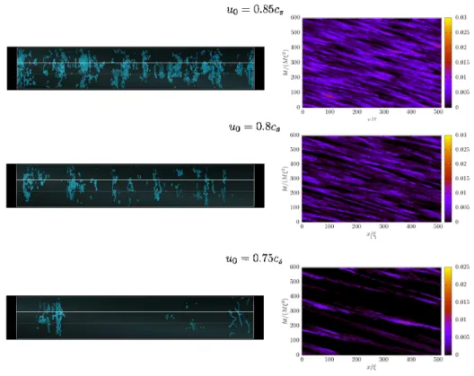
(10) 157. where \mathrm{c}_{s} \sqrt{2g$\rho$_{0}}/M is the sound velocity and N is the total number satisfying |n| \leq 10 and perform the simulation of the GP equation (26) until the system reaches the statistically steady state. After calculating averaged physical values over the time, we continue the simulation with the slightly smaller external current u_{0} \rightarrow u_{0}-0.01c_{s} and obtain the statistically steady state. Repeating these processes, the system finally reaches the vortex‐free state under the some external current which can be regarded as the critical external current from turbulent to vortex‐free states. =. Figure. 3:. dences of. ,. Right panels: Steady snapshots of spatial vortex configurations. Left panels: Depen‐ integrated vortex‐line density over the yz‐plane on the coordinate x and the time t.. Intensities of external currents u_{0}. are. 0.85. (top panels),. 0.8. (middle panels). and 0.75. (lower panels). respectively. Left. configurations with the intensities u_{0}= These three panels show that the system reaches non‐uniform steady turbulent state with finite vortices. With decreasing the intensity u_{0} vortices become non‐uniformly more dilute showing a stripe structure, which indicates there exist repeating of locally turbulent and non‐turUulent states. This feature can be clearly seen in right panels of Fig. 3 which show the dependence of integrated vortex‐line density over yz plane on the coordinate x and t We can see that several turbulent clouds having nonzero vortex 0.75. panels of Fig.. (upper panel),. 3 show. 0.8. snapshots of spatial. (middle panel),. ,. .. and 0:85. vortex. (lower panel)..

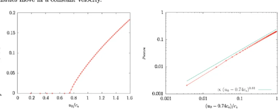
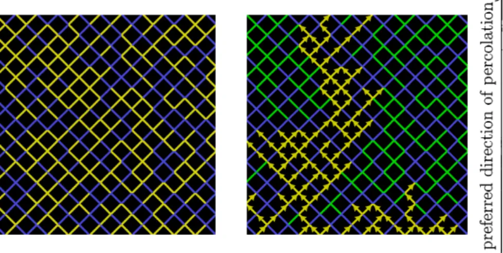
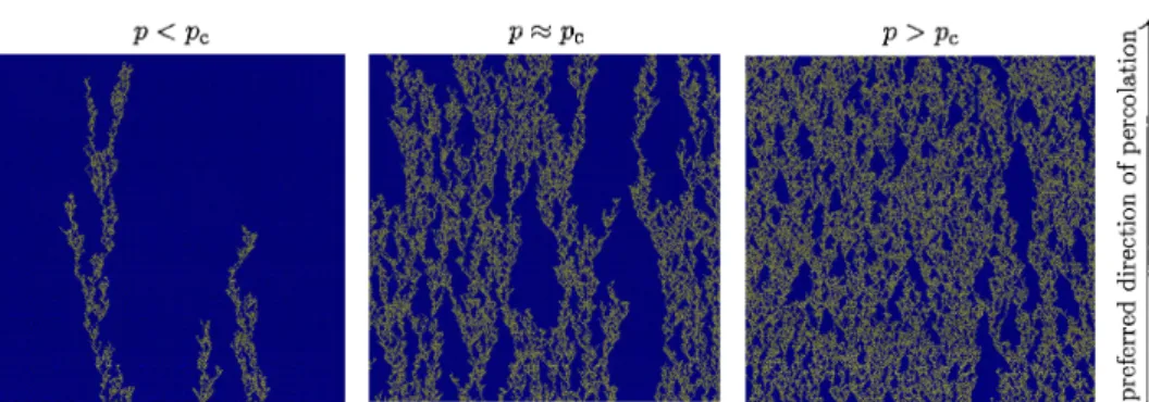
(11) 158. densities. move. in. a. constant. velocity.. Figure 4: Left panel: Vortex‐line density $\rho$_{\mathrm{v}\mathrm{o}\mathrm{r}\mathrm{t}\mathrm{e}\mathrm{x} as a function of the external current u_{0} in a linear scale. Right panel: Vortex‐line density $\rho$_{\mathrm{v}\mathrm{o}\mathrm{r}\mathrm{t}\mathrm{e}\mathrm{x} as a function of the external current u_{0}-0.74c_{\mathrm{s}} in a log‐log scale. Here the value 0.74c_{\mathrm{s}} is the critical external current at which the vortex‐line density $\rho$_{\mathrm{v}\mathrm{o}\mathrm{r}\mathrm{t}\mathrm{e}\mathrm{x} vanishes.. Left. panel. current u_{0}. .. in. Fig.. 4 shows the. The vortex‐line. density. dependence. of the vortex‐line. $\rho$vortex decreases with. density $\rho$_{\mathrm{v}\mathrm{o}\mathrm{r}\mathrm{t}\mathrm{e}\mathrm{x} decreasing the external. on. the external. current u_{0} , and. vanishes at u_{0}\equiv u_{0\mathrm{c}}\simeq 0.74c_{\mathrm{s}} We can expect the transition from quantum turbulence with vortices to vortex‐free state occurs at the critical external current u_{0\mathrm{c} Right panel in Fig. 4 shows the same dependence as the left panel in log‐log scale and the critical behavior of the vortex‐line density as .. .. $\rho$_{\mathrm{v}\mathrm{o}\mathrm{r}\mathrm{t}\mathrm{e}\mathrm{x} \propto (u_{0}-u_{0\mathrm{c} )^{ $\beta$} with the critical exponent $\beta$\simeq 0.81 This result suggests that the obtained transition is non‐equilibrium phase transition with regarding the vortex‐line density $\rho$_{\mathrm{v}\mathrm{o}\mathrm{r}\mathrm{t}\mathrm{e}\mathrm{x} as the order parameter for quantum turbulence phase, The value of the critical exponent $\beta$\simeq 0.81 is .. (3+1) ‐dimensional directed percolation, suggesting that the obtained umiversality class for the directed percolation. Here we briefly review the directed percolation [7]. In Fig. 5, we show examples of ordinary 2‐dimensional bond isotropic percolation and 1+1 ‐dimensional bond directed percolation on a diagonal square lattice. In these models, bonds between adjacent sites of a square lattice are open with probability p and otherwise closed. As shown in the right panel of Fig. 5, there is a specific preferred direction in space. The bonds work as valves in a way that the spreading direction is fixed along the given direction, as indicated by the arrows. As in the case of isotropic percolation, directed percolation exhibits a continuous phase transition. The phase transitions of both isotropic and directed percolations are characterized by an order parameter P_{\infty} which is defined as the probability that a randomly selected site generates an infinite cluster. In finite dimensions 2\leq d< \infty there is a continuous phase transition separating P_{\infty} =0 and P_{\infty} >0 at some critical value p=p_{\mathrm{c}} with 0<p_{\mathrm{c}} < 1 The critical threshold p_{\mathrm{c} for directed percolation is larger than that for isotropic percolation. Numerical simulations of (1+1) ‐dimensional directed bond percolations with different prob‐ ability p are illustrated in Fig. 6. In this figure, we show typical configurations starting from random conditions at the boundary along the preferred direction. Results changes significantly at the phase transition. For p <p_{\mathrm{c}} the number of connecting bonds decreases exponentially along the preferred direction until the system reaches the state with no connecting bonds, whereas for consistent with that for the transition has the. ,. .. ,.

(12) 159. Examples of 2‐dimensional bond isotropic percolation (left panel) and (1+1) ‐dimensional percolation (right panel) on a diagonal square lattice having the same configuration of open and closed bonds. In the left panel, open (closed) bonds are represented by yellow (blue) lines. In the right panel, the percolating direction is restricted to follow the sense of the arrows, leading to a directed cluster of connected sites. Some open bonds in the directed case are, therefore, cannot join in connected clusters as shown with green lines. Figure. 5:. bond directed. p>p_{\mathrm{c}} the number of connecting bonds saturates at some constant value. At the critical point the mean number of connecting bonds decays very slowly and the cluster of connecting bonds remind of fractal structures.. As well. magnetization of the Ising model, the phase transitions of the isotropic percolation by universal scaling laws for the order parameter P_{\infty} as P_{\infty}\propto(p-p_{\mathrm{c} )^{ $\beta$} for p>\mathrm{P}\mathrm{c}, where $\beta$ is a universal exponent and depends on the spatial dimension. The same picture emerges in the directed percolation with the different critical exponent $\beta$ from that for the isotropic percolation. For example, the exponent $\beta$ takes $\beta$\simeq 0.14 0.42, 0.66 for d‐dimensional isotropic percolation with d=2 3, 4, and $\beta$\simeq 0.28 0.58, 0.81 for (d+1) ‐dimensional directed percolation with d=1 2, 3. We consider the relationship between the directed percolation and the transition from quantum turbulent to vortex‐free states. For simplicity, we here assume that the space x and time t are discretized as x_{i\in \mathrm{Z}^{3} and t_{j\in \mathrm{Z} and all discretized spatial points can be separated into those with and without vortices. For example, we can imagine a spatial point with vortices as a spatial point in a turbulent cloud as shown in the lower‐right panel of Fig. 4. We then define the binary function as. the. is characterized. ,. ,. ,. ,. ,. s(x_{i}, t_{j}). as. s(x_{i}, t_{j})=. (35). a large energy gap between states with and without vortices, vortices cannot be nucleated spread due to the external uniform current or disappear due to the dissipation. We give intuitive. There is. but. \left{bginary}{l 0,\mathr{i}\mathr{f}\mathr{}\mathr{}\mathr{e}\mathr{}\mathr{e}\mathr{}\mathr{}\mathr{e}\mathr{v}\mathr{o}\mathr{}\mathr{}\mathr{i}\mathr{c}\mathr{e}\mathr{s}\mathr{}\mathr{}x_i,\ 1mathr{i}\mathr{f}\mathr{}\mathr{}\mathr{e}\mathr{}\mathr{e}\mathr{i}\mathr{s}\mathr{n}\mathr{o}\mathr{v}\mathr{o}\mathr{}\mathr{}\mathr{e}\mathr{x}\mathr{}\mathr{}x_i. \end{ary}\ight..

(13) 160. Figure 6: (1+1) ‐dimensional boundary.. directed bond. percolation starting from random. conditions at the. lower. interpretation of this condition. s(x_{i}, t_{j+1})=. as. \left\{ begin{ar y}{l 1\mathrm{i}\mathrm{f}\sum_{k}s(x_{i}+$\Delta$x_{k},t_{j})>1\mathrm{a}\mathrm{n}\mathrm{d}z(x_{i},t_{j})<p,\ 0\mathrm{o}\mathrm{t}\mathrm{h}\mathrm{e}\mathrm{r}\mathrm{w}\mathrm{i}\mathrm{s}\mathrm{e}, \end{ar y}\right.. (36). neighboring spatial point to x_{i} and \displaystyle \sum_{k}s(x_{i}+ $\Delta$ x_{k}, t_{j}) > 1 means neighboring spatial point with vortices. 0<z(x_{i}, t_{j})<1 is the uniformly distributed random number, and vortices can spread to the nearest sites with the probability p or disappear with the probability 1-p Equation (36) is nothing but the condition for the (3+1)dimensional directed percolation under the correspondence of the preferred direction to the time. If we regard the external current u_{0} and the vortex‐line density $\rho$_{\mathrm{v}\mathrm{o}\mathrm{r}\mathrm{t}\mathrm{e}\mathrm{x} as the probability p and the order parameter P_{\infty} with u_{0} \propto p and $\rho$_{\mathrm{v}\mathrm{o}\mathrm{r}\mathrm{t}\mathrm{e}\mathrm{x} \propto P_{\infty} we obtain $\rho$_{\mathrm{v}\mathrm{o}\mathrm{r}\mathrm{t}\mathrm{e}\mathrm{x} \propto (u_{0}-u_{0\mathrm{c} )^{ $\beta$} which is. x_{i}+ $\Delta$ x_{k}. where. is the nearest. that there is at least. one. .. ,. consistent with. giving. the. numerical result of the transition from quantum turbulent to vortex‐free states critical exponent $\beta$ \simeq 0.81 This result support that the underlying physics for. our. same. .. the transition of the directed states. \mathrm{S}\mathrm{J}' \mathrm{e}. same, and the. percolation and the transition from quantum turbulent to vortex‐free intuitive discussion for quantum turbulence with using Eq. (36) is almost. correct.. 5. Summary. In this. proceeding,. we. discuss two. topics of quantum turbulence comprised of quantized vortices.. The first topic is the energy spectrum of fully developed quantum turbulence under a strong energy injection. Being different from conventional turbulence described by the Navier‐Stokes equation, there exists the. mean inter‐vortex distance \ell as an additional scale in quantum turbulence, and scaling regions of the energy spectrum separated by the wave number \approx 1/P In the small wave‐numUer region, the obtained energy spectrum is consistent with the well‐known Kolmogorov law with the power -5/3 In the higher wave‐numberregion, on the other hand, the obtained energy spectrum is characterized by the power -7/5 which is consistent with the theory for the Kelvin‐wave cascade process of a single vortex line in quantum turbulence. The second topic is the transition from quantum turbulence with vortices to vortex‐free state under a weak energy injection. With decreasing the strength of the energy injection, we observe the. there. are. two. .. ..

(14) 161. continuous transition from quantum turbulent to vortex‐free states. Around the transition point, density can be regarded as the order parameter of the transition, showing its power‐. the vortex‐line. law behavior with the critical exponent. The obtained critical exponent is consistent with that for the (3+1) ‐dimensional directed percolation, which suggests that the underlying physics for the transition from quantum turbulent to vortex‐free states is same as that for the transition of the (3+1) ‐dimensional directed percolation. This consistency between two models can be intuitively. understood. by considering the correspondence of the preferred dimension, probability p for open selected, and the order parameter P_{\infty} for the infinite percolating clusters in the directed percolation to the time, the external current u_{0} and the vortex‐line density $\rho$_{\mathrm{v}\mathrm{o}\mathrm{r}\mathrm{t}\mathrm{e}\mathrm{x} in quantum turbulence, respectively. channels to be. References. [1]. K. H. Bennemann and J. B.. Ketterson, Nover Superfluids (Oxford University Press, Oxford,. England, 2013).. [2]. A. J.. [3]. M.. [4]. C. J. Pethick and H. Smith, Bose‐Einstein Condensation sity Press, Cambridge, England, 2008).. in Dilute Gases. [5]. E. H. Lieb and R.. (2002).. [6]. W. F. Vinen and J. J.. [7]. H.. Legget, Quantum Liquids: Bose Condensation And Cooper Paring Systems (Oxford University Press, Oxford, England, 2006).. Ueda, Fundamentals Singapore, 2010).. and New Írontiers. Seiringer, Phys.. of. in Condensed‐matter. Bose‐Einstein Condensation. Rev. Lett. 88, 170409. (World Scientific,. (Cambridge. Univer‐. Niemela, J. Low Temp. Phys. 128, 167 (2002); E. Kozik and B. Svistunov, Phys. Rev. Lett. 92, 035301 (2004); L. Kodaurova, V. Lvov, A. Pomyalov, and I. Procaccia, Phys. Rev. B90, 094501 (2014). Hinrichsen, Adv. Phys. 49,. 815. (2000)..

(15)