Asymptotic analysis of the modified Bessel function with respect to the parameter

Asymptotic

analysis

of

the

modified Bessel function

with

respect

to

the parameter

K\^oichi

_UCHIYAMA

Department

of

Mathematics,

Sophia University, Tokyo, Japan

1

Introduction

This is an intermediate report of a joint work with William Boyd at Bristol University.

As the work is not yet completed, this talk is given in the author’s responsability.

The aim of this talk is to give

some

observation on adjacency of saddles concerning

hyperasymptotic analysis to the modified Bessel function.

In the paper [3], W.Boyd derived a new representation of the gamma function,

ex-plointing hyperasymptotic analysis, that is, reformulation of the method of steepest de-scents by M. Berry and C. Howls in [1]. There appeared aseries of infinitely many saddles

lying on an adjacent contour in the integral representation of the gamma function. He

expected generalization of his analysis and proposed, as an example, the modified Bessel

function $K_{\nu}(\nu Z)$ when $\nu$ tends to infinity ([3] p628).

In this note, I explain the feature of the

case

of the modified Bessel function, which

turns out to be more complicated than that of the gamma function in [3]. In fact, there

appear two series of infinitely many saddles $w^{(2n)}(Z)$ and $w^{(2n+1}()z),$ $n\in N$. The

fun-damental step in the hyperasymptotic analysis of integrals with saddles is to determine

adjacency of saddles. In this report, our observation on adjacency relies on computer

graphics ofStokes lines and steepest descent

curves.

Our conjectural conclusion is:

The complex $z$-plane is divided into the two regions, the unbounded domain (called

radial) and the bounded domain (called spiral) separated by a piecewise analytic bounded

closed

curve

(Figure $\mathit{2}(b)$)

$1$

$\Re(\sqrt{1+z^{2}}+\log\frac{1-\sqrt{1+z^{2}}}{z})=0$.

(i) Suppose $z$ is in the unbounded (radial) domain. For any

fixed

$p$, only $w^{(\pm 1+)}p(Z)$ are

adjacent to $w^{(p)}(z)$.

(ii) Suppose $z$ is in the bounded (spiral) domain. For any

fixed

$p,$ $w^{(p)}2n+1+(z)$ are

adja-cent to $w^{(p)}(z)$

for

all $n$. $w^{(2n+p}()Z)$ are on the adjacent contour emanating

from

$w^{(p)}(z)$

for

all $n$.

Hyperasymptotic analisys has been developped by M.Berry, C.Howls, W.Boyd, $\mathrm{F}.\mathrm{W}$.J.

1Cf. the eye-shaped domain inOlver’s [7], Chap.10, 8.2, where the asymptotic analysis of themodified

Figure 1: The Stokes lines for vaious phases of$\nu$. The bounded Stokes lines from $i\mathrm{t}\mathrm{o}-i$

for ph $( \nu)=\pm\frac{1}{2}\pi$ are the boundary of the bounded (spiral) and the unbounded (radial)

domains.

Olver, A. Olde Daalhuis and others (See Boyd [4], Howls [6] also the reports given by C.

Howls and A. Olde Daalhuis in this symposium). E. Delabaere (e.g. [5]) gave an

inter-pretation by resurgent function theory. It seems an interesting problem to give rigorous

analysis of this example in view point of hyperasymptotic analysis or resurgent function

theory.

We review the several notations. The modified Bessel function $K_{\nu}(z)$ is the solution

to the equation

(1.1) $\frac{d^{2}K}{dz^{2}}+\frac{1}{z}\frac{dK}{dz}-(1+\frac{\nu^{2}}{z^{2}})K=0$,

defined by $K_{l\text{ノ}}(z)= \frac{\pi}{2}\frac{I_{-\nu}(z)-I_{\nu}(z)}{\sin\nu z}$ with $I_{\nu}(z)=e^{-i\nu\pi}/2J_{\mathcal{U}}(iz)$. When $\Re z$ is positive, it has

an integral representation

(1.2) $K_{\nu}(z)= \frac{1}{2}\int_{-\infty}^{\infty}e^{-\mathcal{U}}-z\mathrm{s}\mathrm{h}{}^{t}dtt\mathrm{c}\mathrm{o}$.

In this paper, we shall discuss the modified Bessel function $K_{\nu}(\nu Z)$ and related variants

for large complex $\nu$ and fixed complex $z$.

Our starting point is the integral reprentation (see e.g. [7] p.250, (8.03)) (1.3) $K_{\nu}( \nu Z)=\frac{1}{2}\int_{-\infty}^{\infty}e^{-\nu}d\{t+z\cosh t\}t$.

This is an integral, as we shall see, with infinite number of saddles The extended method of steepest descents [3], [1] is applicable. On the other hand, ifwe put $F(z)=K_{\nu}(\nu Z)$ for

fixed $\nu,$ $F(z)$ satisfies an second order differential equation

(1.4) $\frac{d^{2}F}{dz^{2}}+\frac{1}{z}\frac{dF}{dz}-\nu^{2}(1+\frac{1}{z^{2}})F=0$,

with a large complex parameter $\nu$. WKB analysis is applicable for asymptotic analysis

These two view points and their interplay are charactersitic in our arguments.

Acknowledgement: The author wish to express his appreciation to members at the

School ofMathematics, Universityof Bristol and also at theLaboratoryofJ.-A. Dieudonn\’e,

University ofNice for their interest and hospitality during his stay on sabbatical leave.

2

Infinite

number of saddles and

their

adjacency

2.1

Saddle points

We rewrite the integral representation of the modified Bessel function (2.5) $K_{\nu}( \nu z)=\frac{1}{2}\int_{-\infty}^{\infty}e^{-\nu p(z}’ w)dw$,

where

(2.6) $p(z, w)=w+z\cosh w$.

We

assume

always $z\neq 0$. This is a phase function of $w$ with a nonzero parameter $z$

and we often omit $z$ to denote it simply by $p(w)$. The equation $p’(w)=0$ reduces to a

quadratic equation of$e^{w}$. We have

(2.7) $e^{w}= \frac{-1+\sqrt{1+z^{2}}}{z}$, $- \frac{1+\sqrt{1+z^{2}}}{z}$_.

Therefore, we have two series of an infinite number of saddles (2.8) $w^{(2n)}$ _$=$ $\log\frac{-1+\sqrt{1+z^{2}}}{z}+2n\pi i$_,

(2.9) $w^{\prime_{\mathit{2}n+1)}}\backslash$

$=$ $\log\frac{1+\sqrt{1+z^{2}}}{z}+(2n+1)\pi i$,

where $n\in N$. We easily see that $p’(w)=p^{;\prime}(w)=0$ if and only if $w=(n+ \frac{1}{2})\pi\dot{i}$ and

$z=(-1)^{n_{i}}$. In this case, $p”(\prime w)=0$ is not satisfied. Hence, $\mathrm{o}\mathrm{n}\mathrm{l}\mathrm{y}\pm_{i}$ are the two double

saddles and the others

are

all simple.

The points $z=\pm_{\dot{i}}$, where two simple saddles coalesce,

are

considered the turning

points also in view point ofsteepest descents method.

We note that $e^{-w}= \frac{1\pm\sqrt{1+z^{2}}}{z}$ with the

same

choice of the double signatures

as

in $e^{w}$.

We call their images by the map $p(\cdot)$ singularities on the complex $\xi$-plane. We have

two series of the infinite number of singularities$p^{(n)}=p(w^{(n)})$: (2.10) $p^{(2n)}$ _$=$ $\log\frac{-1+\sqrt{1+z^{2}}}{z}+\sqrt{1+z^{2}}+2n\pi i$,

(2.11) $p^{(2n+)}1$ $=$ $\log\frac{1+\sqrt{1+z^{2}}}{z}-\sqrt{1+z^{2}}+(2n+1)\pi i$.

We note that

(2.12) $p^{(2n)}+p^{(1)}2m+=(2(n+m)+1)\pi i$.

Conjecture. Any two singulairities $p^{(n)}$ and $p^{(m)}$ for different _$n,$ $m$ do not coalesce on the

2.2

Steepest

descents

For simplicity,

we

omit $z$ in the function$p(z, w)$. We put

(2.13) $\theta=\mathrm{p}\mathrm{h}(\nu)$ and $p^{(n)}=p(w^{(n)})$.

We define

(2.14) $p^{(nm)}=p^{(m)}-p^{(n)}$_, $\theta^{(nm)}=\mathrm{p}\mathrm{h}(p^{(nm)})$.

Following Berry and Howls’s computations in our context (see also Boyd [3]), we

consider

(2.15) $S^{(n)}( \nu)=\nu^{\frac{1}{2}}\int_{C^{(n)}}(\theta)p\exp(-\nu[(w)-p](n))dw$,

where $C^{(n)}(\theta)$ is the path ofsteepest descent for $\theta$ passing through $w^{(n)}$. We define Stokes

lines in view point of steepest descents method by the locus of $\{z\in C;\propto s[\nu p^{(n})(z)]=$

$s^{\infty}[\nu p^{()}m(z)]\}$ for

some

different integers $n$ and $m$. It is readily reduced to the case where

$n$ and $m$ have different parity, say, $n$ is even and $m$ is odd.

Proposition 2.1 Stokes lines in viewpoint

_of

steepest descents method

_satisfies

thesame

differential

relation

_satisfied

by those

_defined

by the $WKB$ method.

We give description of paths of steepest descents. We introduce real variables, $z=$

$x+\dot{i}y$ for the independent variable of the differential equation, $\theta$ for the phase of the

asymptotic parameter $\nu$ and $w=u+iv$ for the integration variable.

Proposition 2.2 Thepaths

_of

steepest descents or ascents $satiSf\sim vthe$

differential

equation

(2.16) $g(u, v)\dot{u}+f(u, v)\dot{v}=0$

where

$f(u, v)$ $=$ $\cos\theta+\frac{1}{2}\{e^{u}(x\cos(\theta+v)-y\sin(\theta+v))$

(2.17) $+e^{-u}(x\cos(\theta-v)-y\sin(\theta-v))\}$ ,

$g(u, v)$ $=$ $\sin\theta+\frac{1}{2}\{e^{u}(x\sin(\theta+v)+y\cos(\theta+v))$

(2.18) $-e^{-u}(X\sin(\theta-v)-y\cos(\theta-v))\}$

.

REMARK 1. If we choose $\beta$ such that $\cos\beta=x/\sqrt{x^{2}+y^{2}}$ and $\sin\beta=y/\sqrt{x^{2}+y^{2}}$,

we

have

(2.19) $f(u, v)$ $=$ $\cos\theta+\frac{\sqrt{x^{2}+y^{2}}}{2}\{e^{u}\cos(\theta+v+\beta)+e^{-u}\cos(\theta-v+\beta)\}$

(2.20) $g(u, v)$ $=$ $\sin\theta+\frac{\sqrt{x^{2}+y^{2}}}{2}\{e^{u}\sin(\theta+v+\beta)-e^{-u}\sin(\theta-v+\beta)\}$ .

REMARK 2. The differential relation is invariant for translation of$2\pi$ in $v$-variable. The

We give approximatedescription ofpaths ofthe steepest

near

simplesaddles by Taylor

expansion. This approximation is used as initial step in the numerical integration of the

differential relation.

Let $w^{(n)}$ be a simple saddle. Then,

$p(w)$ $=p(w^{(n)})+p’(w^{(})n)(w-w^{(n}))+ \frac{p’’}{2!}(w-w^{(})^{2}n)+O((w-w^{(n})^{3}))$

$=p(w^{(n)})+ \frac{(-1)^{n}}{2}\sqrt{1+z^{2}}(w-w^{(})^{2}n)+^{o}((w-w)(n)3)$ _.

Hence, if$w$ in on the locus of$s^{\infty}[p(w)]=\infty s[p(w^{(n)})]$,

we

have approximately,

$\theta+2\mathrm{p}\mathrm{h}(w-w^{(})n)+\mathrm{P}\mathrm{h}(\nu p’(\prime w^{(})n))=m\pi$,

where $m$ is an integer. The linear approximation of the paths of the steepest near

$w^{(n)}$ is

given by

(2.21) $\mathrm{p}\mathrm{h}(w-w^{(})n)=-\frac{\theta}{2}-\frac{\mathrm{p}\mathrm{h}((-1)n\nu\sqrt{1+z^{2}})}{2}+\frac{m}{2}\pi$, $m=0,1,2,3$ ,

which does not depend on $n$ as a set of four lines.

We define the domain $\triangle(n)$. We consider all the steepest-descent paths, for different $\theta$,

which emanate from the saddle point $w^{(n)}$. They sweep out the domain surrounded by

a finite or infinite number of steepest-descent paths $C^{(m)}(-\theta^{(nm)})$ passing through $w^{(m)}$,

called adjacent contour. This domain is denoted by $\triangle(n)$. The saddles $w^{(m)}$ are called

adjacent to the saddle $w^{(n)}$. They

are

hit by the steepest descent path $C^{(n)}(-\theta^{(nm)})$

issuing from the $w^{(n)}$.

2.3

Review of hyperasymptotic representation

We recall the hyperasymptotic formula given by M.Berry-C. Howls [1]. We

use

the

same

notations as in previous sections.

Let $\Gamma^{(n)}$ be

a

finite loop in $\triangle(n)$ surrounding a part of $C^{(n)}$ including the two zeros of

the denominator ofthe integrand.

The basis for hyperasymptotics is the following

resurgence

formula:

(2.22) $S^{(n)}(\nu)$ $=$ $\sum_{r=0}^{N-1}\frac{a_{r}^{(n)}}{\nu^{r}}+R_{N}^{(n)}(\nu)$,

$a_{r}^{(n)}$ _$=$ $\frac{\Gamma(r+\frac{1}{2})}{2\pi\dot{i}}\int_{\mathrm{r}^{(n})}\frac{1}{[p(w)-p^{(}]^{r}n)+1/2}dw$,

$R_{N}^{(n)}(\nu)$ _$=$ $\frac{1}{2\pi i\nu^{N}}\sum_{m}\frac{1}{(p^{(nm)})^{N}}\int_{0}^{\infty}\frac{\sigma^{N-1-\sigma}e}{1-\frac{\sigma}{\nu p^{(nm)}}}s(m)(\frac{\sigma}{p^{(nm)}})d\sigma$,

where $w^{(m)}$

are

adjacent saddles to $w^{(n)}$.

This is a review ofgeneral theory in

our

context.

Proposition 2.3 (2.23) $S^{(2n)}.(\nu)$ $=$ $S^{(0)}(\nu)$ (2.24) $S^{(2n+}1)(\nu)$ $=$ $S^{(1)}(\nu)$ We notice (2.25) $p^{(2}n,2n\pm 1)$ _$=$ $-2p^{(0)}\pm\pi i$, (2.26) $p^{(0,\pm(2}m+1))$ _{$=$ $-2p^{(0)}\pm(2m+1)\pi$.}

In this note, we will not discuss the analytic formulas in detail.

3

Stokes lines

In this section, we discuss Stokes lines of the equation in view point ofWKB analysis. We

assume

the WKB formal expansion

(3.1) $F(z)=e^{-\nu S(}z)n= \sum a(nZ)\nu\infty 0-n$.

Substitutingthis into the equation _{and rearranging the result by the power of}$\nu$, we obtain

the relation of the highest order

(3.2) $\nu^{2}\{(\frac{dS}{dz})^{2}-(1+\frac{1}{z^{2}})\}=0$.

Hence, we have

(3.3) $S(z)= \pm\int_{z_{0}}^{z}\frac{\sqrt 1\overline{+\zeta^{2}}}{\zeta}d\zeta$,

where $z_{0}$ isan arbitrary initial pointexcept the origin. Then wehave _{$a_{0}(z)=C(1+z^{2})^{-1}/4$},

although we do not need it for

our

analysis. We choose $i$ or $-i$

as

$z_{0}$, which is

one

of the

turning. points of the equation and define the Stokes lines from the turning point $z_{0}$. We

consider three cuts on the complex plane, two along a half straight line starting from the

turning points and the other from the origin. We put on this cut plane

(3.4) $S_{j}(z)=(-1)^{j-1} \int_{z}0\frac{\sqrt{1+\zeta^{2}}}{\zeta}d\zeta z$, for $j=1,2$ ,

where $\sqrt{1}=1$ in the integrand. Then, _{Stokes lines of the equation}

issuing from the

turning point $z_{0}$

are

defined

as

the analitically continued locus

(3.5) $\{z\in C;\propto s[\nu S_{1}(z)]=s[\propto\nu S2(_{Z})]\}$,

that is,

where by definition

(3.7) $\theta=\mathrm{p}\mathrm{h}(\nu)$.

Stokes lines

are

locallysmooth curves except the turning points as singularities. Denoting

locally

one

of the Stokes lines by $z(\sigma)$ with

one

dimensional real parameter a, we have a

differential relation of$z(\sigma)$.

Proposition 3.1 Outside the turning points, any analytically continued Stokes line $z(\sigma)$

satisfies

(3.8) $s^{\infty}[e^{i\theta} \dot{z}(\sigma)\frac{\sqrt{1+z(\sigma)2}}{z(\sigma)}]=0$ .

This differentialrelation will be numerically integrated and give graphical imformation

of the Stokes lines. We put

(3.9) $\frac{\sqrt{1+z^{2}}}{z}=P(x, y)+iQ(x, y)$_.

Then the differential relation has the form

(3.10) $\dot{y}(P(x, y)\cos\theta-Q(X, y)\sin\theta)+\dot{x}(P(x, y)\sin\theta Q(x, y)\cos\theta)=0$.

In $(x, y)$-coordinates, the points $(0,1),$ $(0, -1),$ $(0,0)$ are singularities of the vector field,

corresponding to the turning points $z=i,$ $-i$ and the pole $z=0$. All the pictures of

Stokes lines are obtained by approximate integration of the vector field by the

Runge-Kutta method, starting from a small neighbourhood of the turning points.

On the other hand, the $\frac{\sqrt{1+z^{2}}}{z}$ in (3.6) has a primitive

$\sqrt{1+z^{2}}+\log\frac{1-\sqrt{1+z^{2}}}{z}$.

We fix the branches as $\sqrt{1}=1$ and $\log\frac{1-\sqrt{1+z^{2}}}{z}=\mp\frac{\pi}{2}\dot{i}$ when _{$z– \exp(\pm\frac{\pi}{2}i)$}. Therefore,

the equation in (3.6) for $z_{0}=\dot{i}$ is

(3.11) $\propto s[e^{i\theta}(\sqrt{1+z^{2}}+\log\frac{1-\sqrt{1+z^{2}}}{z}+\frac{\pi}{2}\dot{i})]=0$,

and the other one for $z_{0}=-i$ is

(3.12) $\propto s[e^{i\theta}(\sqrt{1+z^{2}}+\log\frac{1-\sqrt{1+z^{2}}}{z}-\frac{\pi}{2}\dot{i})]=0$.

Graphics of Stokes lines from $\dot{i}$ and from $-\dot{i}$ show point-symmetry with respect to the

origin $z=0$. This symmetry reflects that if$z$ satifies the first equation, then $ze^{\pi i}$ satisfies

the (analytically continued around the origin) second equation and that the

converse

is

also true.

We

can

verify analytically several facts

seen

by the figures obtained by numerical

(S1) If $z$ tends to $\infty$ along a Stokes line, $\theta+\mathrm{p}\mathrm{h}(z)$ is asymptotically $0$ or $\pi$ mod $2\pi$.

(S2) Approximate description near the turning points: we have asymptotically

(3.13) $\mathrm{p}\mathrm{h}(z-i)=\frac{\pi}{6}-\frac{2}{3}\theta+\frac{2}{3}n\pi$,

where $n$ is

an

arbitrary integer.

For example, if$\theta=0$, the asymptotic directions ofStokes lines issuing from $\dot{i}$

are

$\frac{\pi}{6},$ $\frac{5}{6}\pi,$ $- \frac{\pi}{2}$.

We have the symmetric result for the case $z_{0}=-i$. They are used as the first step from

the turning points for the numerical integration of the differential relation (3.11).

(S3) Approximate description near the pole is a conformal image ofa logarithmic spiral.

(S4) Existence of finite closed Stokes lines when $\theta=\pm\frac{\pi}{2}$. In this case, the two equations

(3.11) and (3.12) are equal to

(3.14) $\Re[\sqrt{1+z^{2}}+\log\frac{1-\sqrt{1+z^{2}}}{z}]=0$.

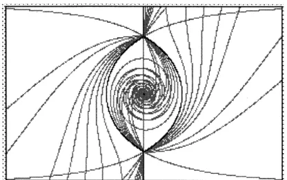
The two Stokes lines connecting $\pm_{i}$ consist of the boundary of a bounded domain. We

call this bounded domain spiral, since it is filled with spiral Stokes lines issuing $\mathrm{f}\mathrm{r}\mathrm{o}\mathrm{m}\pm i$

as $\theta$ changes from $0$ to $\pm\frac{\pi}{2}$ (See Figure 1, Figure $2(\mathrm{b})$). The interior of the complement

will be called radial.

4

Discussion

on

adjacency

Integrating numerically by a simple version of Runge-Kutta method the differential

rela-tions in the previous secrela-tions, we can observe steepest descent curves and Stokes lines by computer graphics $([8])[9])$.

When we follow faithfully the definition of adjacency, we have to verify whether steep-est descent

curves

issuing from one saddle $w^{(n)}$ hit or not another saddle for a certain

phase of$\nu$. Since adjacency of saddles $w^{(m)}$ to $w^{(n)}$ is transformed into visibility between

the corresponding two singularities$p^{(m)}$ and $p^{(n)}$ on the Borel plane, the critical phase of

$\nu$ is the angle $-\theta^{(nm)}$, if the they are on the same Riemann sheet over the Borel plane.

Let the steepest descent $C^{(n)}(-\theta^{(nm)})$ passing through $w^{(n)}$ hit the saddle $w^{(m)}$. This

measns

that we have Stokes phenomenon with respect to $\theta$ near $-\theta^{(nm)}$ while

$z$ is fixed.

The

same

steepest descent picture means also that we have Stokes phenomenon with

respect to $z$ when the phase $-\theta^{(nm)}$ is fixed. Hence, in order to know adjacency, we have

only to verify whether $z$ is

on

the Stokes line by the exact WKB method ([10]) with the

phase $-\theta^{(nm)}$_.

We observe that if$z$ is inside the spiral domain, $z$ is passed over infinitely many times

by spiral Stokes lines when $\theta$ changes from

$0 \mathrm{t}\mathrm{o}\frac{\pi}{2}$ or $\frac{-\pi}{2}$. This must induce infinite number

of adjacent saddles when $z$ is in the spiral domain. On the other hand, the domain outside

Figure 2: (a) and (b).

four times modulo $2\pi$ by the radial Stokes lines issuing from $\pm_{\dot{i}}$ as $\theta$ changes. We

are

convinced of the following conjectural conclusion through the observation of graphics.

(i) Suppose$z$ is in the radial domain. For any

fixed

$p$, only $w^{(\pm 1+p)}(z)$ are adjacent to

$w^{(p)}(_{Z)}$.

$(\dot{i}i)$ Suppose $z$ is in the spiral domain. For any

fixed

$p,$ $w^{(p)}2n+1+(z)$ are adjacent to

$w^{(p)}(z)$

for

all $n$. $w^{(2n+p)}(z)$ are on the adjacent contour emanating

from

$w^{(p)}(z)$

for

all

$n$.

A similar situation to the first case (i) has already appeared in Boyd [2]. The second

situation

seems

new and very much different from the Gamma function

case.

When $z=$

0.662743..

with the phase $\frac{1}{2}\pi$, all saddles are connected by one zig-zag

steepest descent

curve.

This picture recall

us

ofa double Stokes phenomenon $([8],[9])$.

5

Examples

of

adjacent

saddles

5.1

An

example

with

$z$

in

the

unbounded domain:

$z=2$

We take $z=2$ as an example of a point in the

unbounded

domain

To verify adjacency ofsaddles, we don’t need to check all angles. (It is impossible for the computer!) We have only to verify the steepest

curves

when $\theta=\mathrm{p}\mathrm{h}(p^{(mn)})$. Notice

that there exist (

$‘ \mathrm{h}\mathrm{o}\mathrm{r}\mathrm{i}\mathrm{z}\mathrm{o}\mathrm{n}\mathrm{t}\mathrm{a}\mathrm{l}$” steepest descent

curves

prevent from adjacency of saddles

except the pair $w^{(n)}$ and $w^{(n\pm 1)}$. The

reason

why $w^{(n)}$ is adjacent only to $w^{(n\pm 1)}$ is

seen

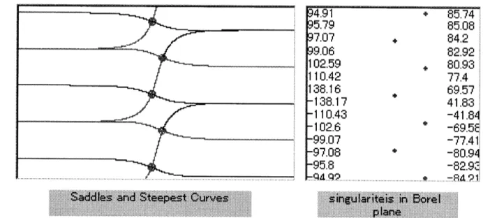
by the fact that the point $z=2$ is exactly on a Stokes line $\mathrm{f}\mathrm{o}\mathrm{r}\pm\theta^{(n\pm 1,n)}$

i.e. $\pm 41.83$ and

$\pm 138.16\deg$ (rounded).

Here,

we

have approximately

$w^{(0)}$ _$=$ $\log\frac{-1+\sqrt{5}}{2}=-0.481211825$,

Figure 3: The left shows the point $z=2$ is exactly on the radial Stokes line for $\theta=$

41.84$\deg$ (rounded). The right is the image of the saddleson the Borelplane. The figures

in the right box are degrees of the angle between the singularities.

Figure 4: The left is a figure of saddles and steepest

curves

for $\theta^{(n,n-1}$)

$=$

-41.84

$\deg$

(round) when $z=2$. The right is the image ofthe saddles onthe Borel plane. The figures in the right box

are

$\mathrm{d}\mathrm{e}\mathrm{g}$

.rees

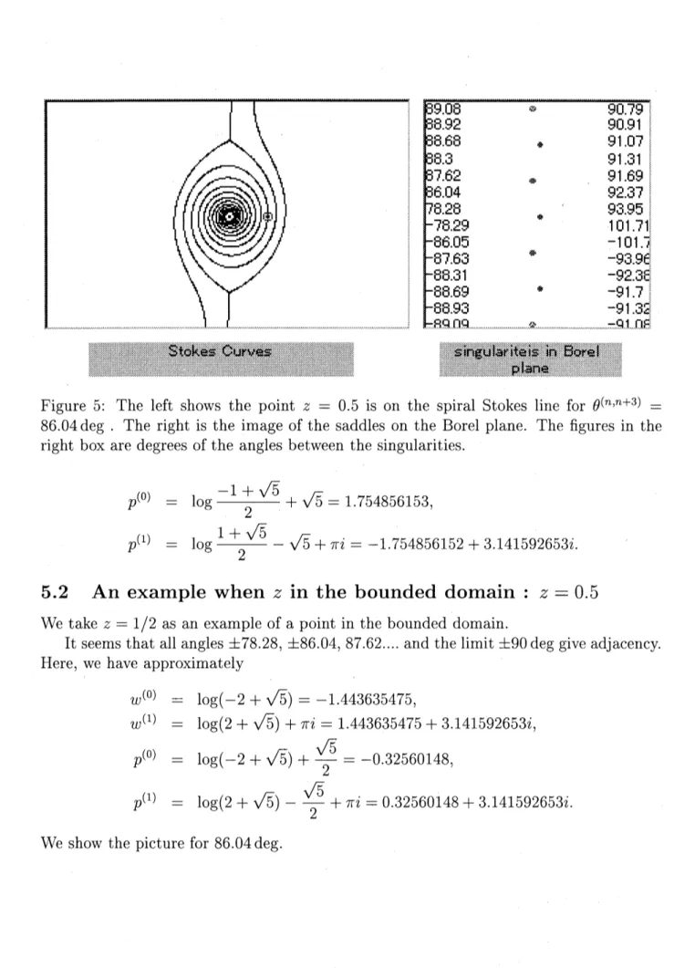
of the angle between the singularities.

Figure 5: The left shows the point $z=0.5$ is on the spiral Stokes line for $\theta^{(n,n+3}$) _$=$

86.04$\mathrm{d}\mathrm{e}\mathrm{g}$

.

The right is the image of the saddles on the Borel plane. The figures in the

right box are degrees of the angles between the singularities.

$p^{(0)}$ _$=$ $\log\frac{-1+\sqrt{5}}{2}+\sqrt{5}=1.754856153$,

$p^{(1)}$ _$=$ $\log\frac{1+\sqrt{5}}{2}-\sqrt{5}+\pi\dot{i}=-1.754856152+3.141592653\dot{i}$.

5.2

An

example when

$z$

in

the bounded domain

:

$z=0.5$

We take $z=1/2$ as an example of a point in the bounded domain.

It seems that all $\mathrm{a}\mathrm{n}\mathrm{g}\mathrm{l}\mathrm{e}\mathrm{s}\pm 78.28,$ $\pm 86.04$, 87.62.... and the$\mathrm{l}\mathrm{i}\mathrm{m}\mathrm{i}\mathrm{t}\pm 90\deg$ give adjacency.

Here, we have approximately

$w^{(0)}$ _$=$ $\log(-2+\sqrt{5})=-1.443635475$,

$w^{(1)}$ _$=$ $\log(2+\sqrt{5})+\pi i=1.443635475+3.141592653i$, $p^{(0)}$ _$=$ $\log(-2+\sqrt{5})+\frac{\sqrt{5}}{2}=-0.32560148$,

$p^{(1)}$ _$=$ $\log(2+\sqrt{5})-\frac{\sqrt{5}}{2}+\pi i=0.32560148+3.141592653i$.

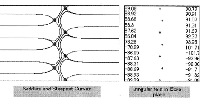
Figure6: The left is afigure of saddles andsteepest curvesfor $\theta^{(n,n+)}\mathrm{s}=86.04\deg$ (roughly

rounded). Thesteepest descents creep up from the saddles $w^{(n)}$ to hit the adjacent saddles $w^{(n+3)}$_.

A

Transcendental

equations

Conjecture. Any two singulairities$p^{(n)}$ and $p^{(m)}$ for different

$n,$ $m$ do not coalesce on the

$\xi$-plane, when $z\neq\pm i$.

More precisely, we put cuts in $z$-plane from $i$ to $\infty$ and from _$-i$ to $\infty$ along the

imaginary axis to uniformize $\sqrt{1+z^{2}}$ with $\sqrt{1}=1$. We should consider the possibility $p^{(2n)}=p^{(1)}2m+$ for some integers $n$ and $m$. It means

$\log\frac{-1+\sqrt{1+z^{2}}}{-1-\sqrt{1+z^{2}}}+2(n-m)\pi i+2\sqrt{1+z^{2}}=0$_,

which is equivalent to

$2\sqrt{1+z^{2}}-2-Z^{2}=z^{2}e^{-2\sqrt{1+z^{2}}}$_. By change of variable $s=\sqrt{1+z^{2}}$_, this is

$(s^{2}-1)e^{-}+2(_{S^{2}+}4S1)e-2S+(S^{2}-1)=0$_,

which reduces to the equation

(A. 1) $(s+\tanh s)(s-\tanh_{S)}=0$.

Our conjecture is that $s=0$ _is a _{unique solution of} $(\mathrm{A}.1)_{\mathrm{C}\mathrm{O}}\mathrm{r}\mathrm{r}\mathrm{e}\mathrm{s}\mathrm{P}^{\mathrm{o}}\mathrm{n}\mathrm{d}\mathrm{i}\mathrm{n}\mathrm{g}$ to $z^{2}=-1$.

References

[1] M.Berry and C.Howls, Hyperasymptotics for integrals with saddles, Proc. R. Soc.

[2] W. Boyd, Error bounds for the method of steepest descents, Proc. R. Soc. London

A 440,(1993),

493-518.

[3] W. Boyd, Gamma function asymptotics by an extension of the method of steepest

descents, Proc. R. Soc. London A 447, (1994),

609-630

[4] W. Boyd, Recent developments in asymptotics obtained via integral representations

of

Stieltues-transform

type, RIMS Kokyuroku 968, (1996), 1-30

[5] E. Delabaere Un peu d’asymptotique, Lecture Note at University of Nice

Sophia-Antipolis, DEA

96-97

[6] C.J. Howls, An Introduction to Hyperasymptotics using Borel-Laplace Transforms,

RIMS Kokyuroku 968, (1996), 31-48

[7] F.W.J. Olver Asymptotics and special functions, Academic Press, 1974, 2nd version

1997, New York

[8] K. Uchiyama, On examples of Voros analysis in complex WKB theory, “M\’ethodes

r\’esurgentes’’ ed. by L. Boutet de Monvel, Hermann, 1994,

115-134.

[9] K. Uchiyama, Graphical illustration ofnew Stokes line for integrals with saddles. An

informal seminar in the workshop ”Exponential Asymptotics” at Cambridge, 1995,

March

[10] A. Voros, The return of the quarticoscillator, The complexWKBmethod, Ann. Inst.