Theoretical and numerical studies of the shallow water equations with a transmission boundary condition
著者 エムディ マスム ムシェド
著者別表示 Md Murshed Masum journal or
publication title
博士論文本文Full 学位授与番号 13301甲第5003号
学位名 博士(理学)
学位授与年月日 2019‑09‑26
URL http://hdl.handle.net/2297/00056470
Creative Commons : 表示 ‑ 非営利 ‑ 改変禁止 http://creativecommons.org/licenses/by‑nc‑nd/3.0/deed.ja
Theoretical and numerical studies of the shallow water equations with a
transmission boundary condition
Graduate School of
Natural Science & Technology Kanazawa University
Division of Mathematical and Physical Sciences
Student ID No. : 1624012011
Name : Murshed Md Masum
Chief Advisor : Professor Masato Kimura
Date of Submission (Revised version) : June 28, 2019
Dissertation
I would like to dedicate this thesis to my loving parents . . .
Acknowledgements
I would like to express my deep sense of gratitude and thanks to my supervisor Professor Dr. Masato Kimura and my co-supervisor Associate Professor Dr. Hirofumi Notsu for their continuous guidance in this whole work. I would like to thank you both from my heart because without your help and support this work was impossible for me. I would also like to thank Mr. Kouta Futai for his help in coding LG-Scheme. I would like to thank Professor H. Kanayama for his kind help in this work. This work would not be possible without the support from Japanese government (Monbukagakusho: MEXT) scholarship. I would also like to thank to the committee members of my thesis. A special thanks to my family. I am grateful to my parents for all of the sacrifices that you’ve made on my behalf. Your prayer for me was what sustained me thus far. I would also like to thank to Sabana Begum my beloved wife. Thank you for supporting me for everything, and especially I can’t thank you enough for encouraging me throughout this experience. To my beloved daughter Maria Murshed and sons Shahrier Murshed and Shams Murshed I would like to express my thanks for being such good children. Finally, I thank my Allah(God) for helping me to finish this work.
Abstract
In this work, the stability of the shallow water equations (SWEs) with a transmission boundary condition is studied theoretically and numerically using a suitable energy. In the theoretical part, using a suitable energy, we begin with deriving an equality which implies an energy estimate of the SWEs with the Dirichlet and the slip boundary conditions.
For the SWEs with a transmission boundary condition, an inequality for the energy estimate is proved under some assumptions to be satisfied in practical computation. In the numerical part, based on the theoretical results, the energy estimate of the SWEs with a trans- mission boundary condition is confirmed numerically by a finite difference method (FDM) and Lagrange–Galerkin method (LGM). The choice of a positive constantc0used in the trans- mission boundary condition is investigated additionally. Furthermore, we present numerical results by a LGM, which are similar to those by the FDM.
The computation of the SWEs with the transmission boundary condition are also made for the Bay of Bengal by a LGM with the triangular mesh. To see the performance of the LGM we have investigated the experimental order of convergence for the LGM with a suitable choice of exact solutions for five different cases of boundary setting for the normsl∞−L2, l∞−H01,l∞−H1,l2−L2,l2−H01andl2−H1. The experimental order of convergence ofu1 andu2isO(h)for all the six norms and experimental order of convergence ofη isO(h)for the normsl∞−L2andl2−L2and for the other four norms experimental order of convergence is notO(h)but confirmed to be convergent.
viii
In order to see whether the transmission boundary condition is independent of its position or not, simulations are made in the Bay of Bengal, setting the transmission boundary condition in two different places. We have computed the mass andL2-norm ofηand the results shows that the transmission boundary condition works well numerically it is almost independent of its position.
The theoretical results along with the numerical results strongly recommend that the transmission boundary condition is suitable for the boundaries in the open sea.
In this work, we have succeeded to give some theoretical results and this is the first step of mathematical foundation of the SWEs with the transmission boundary condition.
Table of contents
List of figures xi
List of tables xiii
1 General introduction 1
2 Derivation of the model equations 13
2.1 SWEs . . . 13
2.2 Surface and bottom boundary conditions . . . 15
2.3 Vertically integrated equations . . . 15
3 Theoretical results 25 3.1 Statement of the problem . . . 25
3.2 Energy estimate . . . 27
4 Numerical results by FDM 35 4.1 Problem setting . . . 35
4.1.1 A finite difference scheme . . . 36
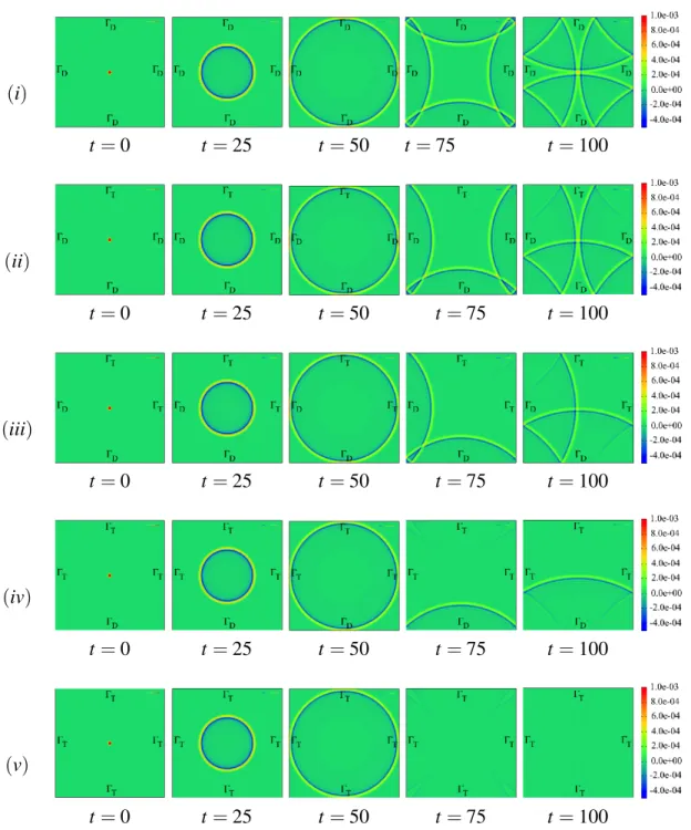
4.1.2 Numerical results for five cases of boundary settings . . . 36
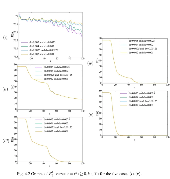
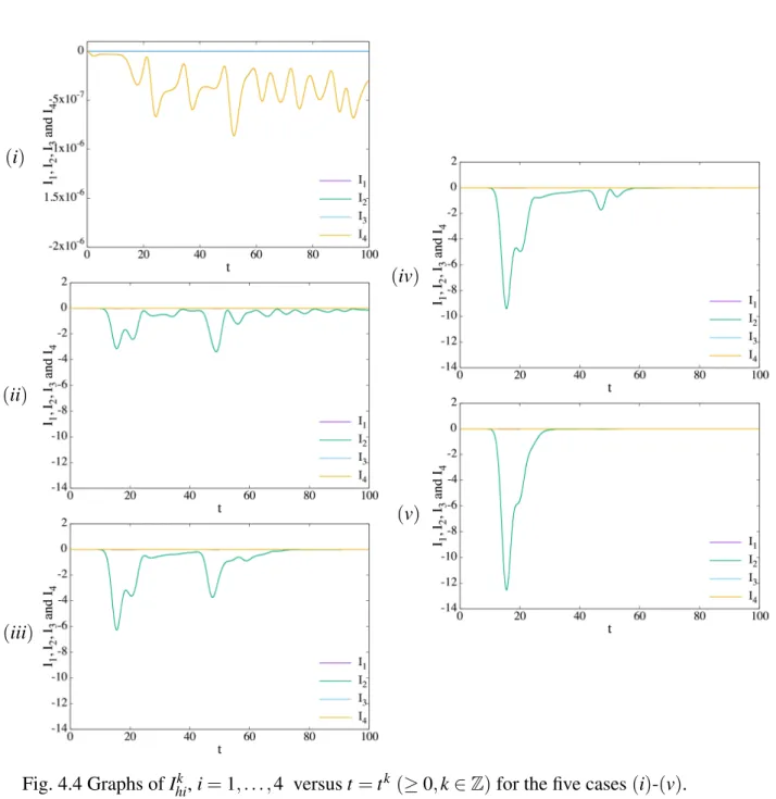
4.1.3 Numerical study of energy estimate . . . 37
4.1.4 Choice ofc0 . . . 43
x Table of contents
5 Numerical results by LGM 45
5.1 LG scheme . . . 45
5.1.1 Numerical results for five cases of boundary settings . . . 46
5.1.2 Numerical study of energy estimate . . . 48
5.1.3 The experimental order of convergence of the LG scheme . . . 52
5.2 Numerical results for the Bay of Bengal . . . 59
5.2.1 Computation of mass andL2norm for the Bay of Bengal . . . 64
6 Instability on the transmission boundary and some future works 69 6.1 Instability on the transmission boundary . . . 69
6.2 Some future works . . . 71
7 Conclusion 73
References 77
List of figures
1.1 The northern part of Bay of Bengal including the coast of Bangladesh, east
coast of India and west coast of Myanmar . . . 2
1.2 Simulation of SWEs in the Bay of Bengal . . . 3
1.3 The northwest corner of Bay of Bengal, and track of several cyclones . . . 5
1.4 A triangular mesh for the Bay of Bengal . . . 9
2.1 Shallow water model domain . . . 14
4.1 Simulated results in a square domain by FDM . . . 38
4.2 Figure showing energy computed using FDM . . . 40
4.3 Figure showing derivative of energy computed using FDM . . . 41
4.4 Figure showingI1,I2,I3andI4computed using FDM . . . 42
5.1 Simulated results in a square domain by LGM . . . 47
5.2 Figure showing energy computed using LGM . . . 49
5.3 Figure showing derivative of energy computed using LGM . . . 50
5.4 Figure showingI1,I2,I3andI4computed using LGM . . . 51 5.5 Figure representing the experimental order of convergence byl∞ L2
norm 53
5.6 Figure representing the experimental order of convergence byl∞ H01
norm 54 5.7 Figure representing the experimental order of convergence byl∞ H1
norm 55 5.8 Figure representing the experimental order of convergence byl2 L2
norm 56
xii List of figures 5.9 Figure representing the experimental order of convergence byl2 H01
norm 57
5.10 Figure representing the experimental order of convergence byl2 H1
norm 58
5.11 A figure of Bay of Bengal domain showing the boundary setting . . . 59
5.12 A figure of Bay of Bengal domain (extended) showing the boundary setting 60 5.13 Simulation in the Bay of Bengal at timet =0s, 2800sand 3120s. . . 62
5.14 Simulation in the Bay of Bengal at timet =3240s, 3740s, 3940sand 4660s. 63 5.15 Figure showing mass ofη . . . 64
5.16 Graph ofη on transmission boundary at timet=0s, 2800sand 3120s . . . 66
5.17 Graph ofη on transmission boundary at timet =3240s, 3740s, 3940sand 4660s . . . 67
5.18 Figure showingL2norm ofη . . . 68
6.1 Graph ofη on transmission boundary at timet=6500s . . . 70
6.2 L2norm ofη for the two cases of transmission boundary setting . . . 70
List of tables
1.1 Table showing the number of deaths associated with several deadly disasters occurred in the Bay of Bengal region . . . 6 4.1 Table showing maximum and minimum values ofI1,I2,I3andI4computed
using FDM . . . 39 4.2 Table showing the values ofc0andSh(c0) . . . 44
Chapter 1
General introduction
Most of the natural phenomena are expressed by partial differential equations or a system of partial differential equations. The Navier-Stokes equations are a system of partial differential equations which expresses a lot of real world phenomena related to fluid flow problems.
According to [24], the equations (Navier-Stokes equations) cannot be solved analytically in most cases due to complicated geometries, initial conditions, boundary conditions or source terms. For this reason, numerical methods are applied, which can be very time consuming.
But under the assumption of a hydro-static pressure distribution one space dimension of the Navier-Stokes equations can be eliminated without much loss of accuracy. This can be done if the fluid is at rest, but in many cases it is sufficient that the horizontal scales are much larger than the vertical scales. The resulting system of partial differential equations is called shallow water equations (SWEs). The reduction of one space dimension reduces the computational cost of numerical solutions greatly. It is pertinent to mention here that the SWEs were first formulated by the mathematician Adh ´emar Jean Claude Barr ´ede Saint- Venant for one-dimensional unsteady open channel flows (see [46] ), and the 1D equations are therefore also known as the Saint-Venant system. After that a lot of developments of the SWEs are done by many researchers for various purpose. The derivation of one-layer viscous SWEs can be found in [21] and two-layers SWEs are derived in [20] for Tsunami simulation purpose. It is of interest to note here that the SWEs are used for the simulation
2 General introduction of Tsunami/storm surge in the bay, e.g., [7, 9–18, 20, 29–33, 35–37, 40–44, 47, 49, 50].
In such simulation there are some boundaries in the open sea (see Figure 1.1). In a real situation, if wave propagates towards such boundaries in the open sea, then there should not be any reflection on these boundaries. Therefore, in the simulation a special type of boundary condition should be imposed on these boundaries which has capability of removing the artificial reflection. In this study, following [20] a transmission boundary condition has been used on the boundaries in the open sea which is capable to remove these kinds of artificial reflection and on the closed boundaries (boundaries in the coast) zero Dirichlet boundary condition is used. Figure 1.2 gives an idea of wave propagation in the Bay of Bengal with the transmission and Dirichlet boundaries.
Fig. 1.1 The northern part of Bay of Bengal including the coast of Bangladesh, east coast of India and west coast of Myanmar.
3
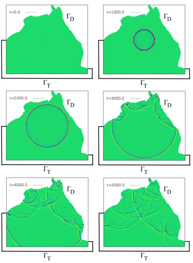
Fig. 1.2 Simulation of SWEs in the Bay of Bengal with transmission and Dirichlet bound- ary conditions, here ΓT and ΓD represent the transmission and the Dirichlet boundaries, respectively
4 General introduction It is of interest to note here that our final goal is to develop a storm surge prediction model for the Bay of Bengal region (see Figure 1.1). The reason of choosing this problem is discussed below.
The coast of Bangladesh is affected by various environmental hazards. Storm surge is one of them, which causes a tremendous loss of lives and properties every year. Table 1.1 lists the number of deaths associated with several deadly disasters occurred in the Bay of Bengal region. The track of different storm surges are presented in Fig. 1.3 for making understand of frequent visiting. As in [34], every year on an average 5–6 storms form in this region, which causes 80% of global casualties. The coastal region of Bangladesh is the most vulnerable because of the shallowness of the coastal water, high density of population in low-lying islands, high bending of the boundaries of the coasts and islands, discharge from river, high range of astronomical tide and favorable track of cyclones (see [8]). In addition, the rates of erosion and accretion are very high in this region. The discharge of sediment is the highest and the discharge of freshwater is the third highest from the river Meghna among all river systems in the world (see [26]). Bangladesh, is situated at the northern tip of the Bay of Bengal between 20◦N to 26◦N Latitudes and 88◦E to 92◦E Longitudes. It is bordered on the west, north and east by India, on the south-east by Myanmar, on the south by the Bay of Bengal. A proper warning system for the region can mitigate the sufferings of its people and live stocks resulting from these storm surges. Though, Bangladesh Meteorological Department (BMD) has a warning system which was bought from IIT, by which they can predict the information of landfall time, sea level rising in a certain accuracy as well as they can predict the storm track but not unique with actuality. Thus an effective storm surge prediction model is highly desirable for the coastal region of Bangladesh which can minimize the resulting damage from storm surges.
5
Fig. 1.3 The northwest corner of Bay of Bengal, and track of several cyclones (source:
http://en.banglapedia.org/index.php?title=Cyclone).
6 General introduction Table 1.1 Storm surge locations and losses of life (data sources: [6, 8] and NASA website).
Year Location Death 1970 Bangladesh 500,000
1737 India 300,000
1897 Bangladesh 175,000 1991 Bangladesh 140,000 1876 Bangladesh 100,000
1864 India 50,000
1833 India 50,000
1822 Bangladesh 40,000
1839 India 20,000
1789 India 20,000
1965 Bangladesh 19,279 1963 Bangladesh 11,520 1961 Bangladesh 11,468
1977 India 10,000
1960 Bangladesh 5,149 2007 Bangladesh 3,376
2009 India 275
2016 Bangladesh 24 2017 Bangladesh 18
Many analyses have been made in prediction of water level during storm surges as well as in development of warning system on the basis of operational forecasting model all over the world, among them worth mentioning studies are [10–15, 47, 50].
A limited number of studies have been done over the Bay of Bengal region considering the west coast of India along with the coast of Bangladesh. Among them some worth mentioning studies are [7, 9, 16–18, 29–33, 35–37, 40–44, 49].
Almost all of the of the studies mentioned here have been conducted using radiation type boundary condition for the boundaries in the open sea, which is very similar to the transmission boundary condition (1.2). Also these studies are about the development of nu- merical computation without ensuring the stability of the model with this kind of boundaries mathematically. It is of interest to note here that for linearized SWEs, the existence and uniqueness of solutions are studied in [22] and the convergence of a finite element scheme
7
for that linearized SWEs is studied in [23]. As far as we know, there is no theoretical results for the existence, uniqueness or regularity for the SWEs with the transmission boundary condition. It is to be noted here that the energy estimate of the SWEs have been studied theoretically in [21] consideringu·n=0. However, as far as we know, there is no theoretical results on the energy estimate of the SWEs with the transmission boundary condition. In this study, we have intended to investigate the stability of the SWEs with the transmission boundary condition both theoretically and numerically through suitable energy estimates.
The SWEs can be considered as a coupled system of a pure convection equation for the function φ of total wave height and a simplified Navier–Stokes equation for the velocity u= (u1,u2)T obtained by averaging function values inx3-direction. LetΩ⊂R2be a bounded domain andT a positive constant. We consider the problem : find(φ,u):Ω×[0,T]→R×R2 such that
∂ φ
∂t +∇·(φu) =0 inΩ×(0,T), ρ φ
h∂u
∂t + (u·∇)ui
−2µ∇·(φD(u)) +ρgφ∇η=0 inΩ×(0,T),
φ =η+ζ inΩ×(0,T),
(1.1)
The explanation aboutu,φ,η andζ can be found in Chapter 3 and in the Figure 2.1. It is known that a boundary data forφ is necessary on the so-called inflow boundary, where u·n<0 is satisfied for the outward unit normal vectorn. We can easily know whether the Dirichlet data for φ is required or not on the Dirichlet and the slip boundaries for u, since the sign of u·nis known a priori. On the transmission boundaryΓT, however, the boundary condition foruandφ is mysterious and problematic from both computational and mathematical view points. The transmission boundary condition of the form
u=cη φ
n onΓT×(0,T), (1.2)
8 General introduction is often used onΓT, wherec(x)is a given positive function andη(x,t) =φ(x,t)−ζ(x)is the elevation from the reference height for a given depth functionζ. It is of interest to note here that including wind stress, bottom friction and Coriolis force in (1.1) a storm surge prediction model can be developed (see (2.11) and (2.12) in Chapter 2). For the theoretical study we set each of them as zero to make the problem simple.
Letφhkandukh be the approximations ofφk: =φ(·,tk)anduk: =u(·,tk), respectively, wheretk: =k∆t(k∈Z)for a time increment∆t. In our computation we getφhk+1by using ukh, and thenuk+1h by using the condition (1.2) as the Dirichlet boundary condition foru. But at the same time we should consider (1.2) as the boundary data forφhk+1if the position is on inflow boundary, i.e.,uk+1h ·n<0. In fact, ifuk+1h ·n<0, we need to give the value ofφhk+1 which is unknown.
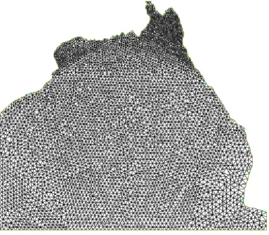
It is known that the finite difference method (FDM) is suitable for a domain of rectangular or square shape, but the real domain is not usually of rectangular or a square shape. It is also known that the finite element method (FEM) is more appropriate for a domain of irregular shape. It is to be noted here that both rectangular and triangular mesh are used for FEM but triangular mesh is more suitable for a domain of complex shape. Considering this fact into account the computation of the SWEs with the transmission boundary condition are also made by a Lagrange–Galerkin method (LGM) with the triangular mesh (see Figure 1.4).
The LGM is a FEM based on the time discretization of the material derivative, φk+1(x)−φk(x−uk(x)∆t)
∆t .
The LGM is a powerful numerical method for the Navier-Stokes equations in fluid flow problems. The study of LGM for the Navier-Stokes equations can be found in , e.g.,[1–
4, 27, 28, 38, 39, 48]. In this study we have used LGM for SWEs.
It is to be noted here that the positionx−uk(x)∆t is the so-called upwind point ofxwith respect touk. In the computation the “nearest” boundary value ofφk is used if the upwind
9
Fig. 1.4 A triangular mesh for the Bay of Bengal
point places outside the domain, and the LGM works without boundary data forφk+1even if uk+1·n<0. In the LG method the problem on the transmission boundary seems to be solved numerically, but it is still problematic mathematically.
In this work, in order to understand the transmission boundary condition mathematically, we study the stability of the SWEs in terms of a suitable energy, and confirm the stability numerically by both FDM and LGM. It is to be noted here that we can show a (successful) energy estimate of the SWEs, when only the Dirichlet and the slip boundary conditions are employed, cf. Corollary 3.2.3-(ii), where such discussions have been done under the periodic boundary condition, e.g., [5, 25].
The stability is considered theoretically with respect to the energy as follows. Introducing a suitable energy, we begin with deriving an equality that the time-derivative of the energy consists of four terms, where three terms are line integrals over the boundary and the other term is an integral over the whole domain which is always non-positive, cf. Theorem 3.2.1.
Since the three line integrals vanish over the Dirichlet and the slip boundaries, as a result, we have the three line integrals over the transmission boundary and the integral over the domain,
10 General introduction cf. Corollary 3.2.3-(i). An energy estimate is obviously obtained if there is no transmission boundary, cf. Corollary 3.2.3-(ii). In addition, we obtain that a sum of two line integrals over the transmission boundary is non-positive under some conditions to be satisfied in real computations, cf. Theorem 3.2.4. Although, at present, the mathematical results do not derive the stability estimate of the SWEs with the transmission boundary condition directly, we have good information and can study the stability numerically by using the theoretical results.
Though our final goal is to develop a storm surge prediction model for the Bay of Bengal region, until now we are not succeeded, but we have some good results, which we believe can help to develop an appropriate storm surge prediction model for that region. We have a theoretical (successful) energy estimate of the SWEs, with the Dirichlet and the slip boundary conditions and a numerical (successful) energy estimate of the SWEs, with the Dirichlet and the transmission boundary conditions by both FDM and LGM. To see the performance of the LGM we have investigated the experimental order of convergence for the LGM with a suitable choice of exact solutions for five different boundary setting (see Section 4.1) for the normsl∞−L2,l∞−H01,l∞−H1,l2−L2,l2−H01andl2−H1. The experimental order of convergence ofu1andu2isO(h)for all the six norms and experimental order of convergence ofη isO(h)for the normsl∞−L2andl2−L2 and for the other four norms experimental order of convergence is notO(h)but confirmed to be convergent. In order to see whether the transmission boundary condition is independent of its position or not, simulations are made in the Bay of Bengal, setting the transmission boundary condition in two different places.
We have computed the mass andL2-norm ofη and the results shows that the transmission boundary condition is almost independent of its position.
As far as we know, there is not a single model using LGM, for the prediction of storm surge in the Bay of Bengal, therefore we strongly believe that our results will be helpful to
11
develop an appropriate storm surge prediction model using LGM for the Bay of Bengal in the near future.
The rest of the thesis is organized as follows:
Derivation of the model equations is presented in Chapter 2. Theoretical study of the energy estimates is presented in Chapter 3. Numerical results obtained by FDM is presented in chapter 4. Numerical results obtained by LGM is presented in chapter 5. In Chapter 6, Instability on the transmission boundary and some future works are given. In Chapter 7, conclusion is given. Finally, the total bibliography that has been needed for completing this thesis is presented.
Chapter 2
Derivation of the model equations
In this Chapter we have derived our model equations following [19] by considering one-layer viscous SWEs.
2.1 SWEs
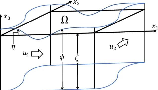
For any atmospheric or oceanic phenomenon, if the horizontal length scale is much larger than the vertical scale, then thex3component of the momentum equation may be approximated by the hydro-static equation. The water depth is considered very smaller than the horizontal length scale and there is the shallow-water low-frequency flow. First, we will derive the viscous SWEs. we consider orthogonal coordinates [m], where the directions in the horizontal plane are represented byx1and x2, respectively , and the vertical direction is represented byx3( see Fig. 2.1). Here t represents time [s]. We have formulated the system using the Navier-Stokes equations assuming hydro-static pressure and gravity in thex3direction, and Coriolis forces occurring in thex1andx2directions.
3
∑
j=1
∂
∂xjuj=0, (2.1)
14 Derivation of the model equations
Fig. 2.1 Shallow water model domain
∂u1
∂t +
3
∑
j=1uj ∂
∂xju1=−1 ρ
∂p
∂x1+1 ρ
3 j=1
∑
∂
∂xjτ1j+f u2, (2.2)
∂u2
∂t +
3
∑
j=1uj ∂
∂xju2=−1 ρ
∂p
∂x2+1 ρ
3 j=1
∑
∂
∂xjτ2j−f u1, (2.3)
0=−ρg− ∂p
∂x3. (2.4)
In the xi (i =1, 2, 3) direction velocity [m/s]is represented by ui(x1,x2,x3,t), pressure [N/m2]is denoted by p(x1,x2,x3,t), density[kg/m3]is denoted byρ, stress[N/m2]in the directionxiacting on thexj plane is denoted byτi j(x1,x2,x3,t), the Coriolis coefficient[1/s]
is denoted by f and the acceleration[m/s2]due to gravity is denoted byg. In addition, the free surface elevation is denoted byη(x1,x2,t), and−ζ(x1,x2)represents the ordinate the bottom boundary surface of the water.
2.2 Surface and bottom boundary conditions 15
2.2 Surface and bottom boundary conditions
There is no velocity component in the normal direction on the water’s free surface plane, and water bottom plane, and so the following conditions are used foru3.
u3= ∂ η
∂t +
2 j=1
∑
uj∂ η
∂xj, (x3=η(x1,x2,t)) u3=−
2 j=1
∑
uj∂ ζ
∂xj, (x3=−ζ(x1,x2)).
(2.5)
2.3 Vertically integrated equations
We integrate each of the equations (2.1), (2.2) and (2.3) with respect tox3, from the ocean floor−ζ(x1,x2)to the water surfaceη(x1,x2,t). Then, the viscous shallow water equations are derived that express averaged rates for the fluid layer. Thus, the velocity component in thexi(i=1, 2)direction averaged over the fluid layer is taken asUi(x1,x2,t). The thickness of the fluid layer is denoted by φ(x1,x2,t). We consider fluids with the constant density represented byρ. φ andUiare represented by the following equations;
φ(x1,x2,t) =η(x1,x2,t) +ζ(x1,x2),
Ui(x1,x2,t) = 1 φ
Z x3=η(x1,x2,t) x3=−ζ(x1,x2)
uidx3.
The integration of (2.1) fromζ(x1,x2)toη(x1,x2,t)in thex3direction yields
0 =
3
∑
j=1Z x3=η(x1,x2,t) x3=−ζ(x1,x2)
∂
∂xjujdx3
=
2
∑
j=1Z x3=η(x1,x2,t) x3=−ζ(x1,x2)
∂
∂xjujdx3+
Z x3=η(x1,x2,t) x3=−ζ(x1,x2)
∂
∂x3u3dx3
16 Derivation of the model equations
=
2
∑
j=1
∂
∂xj
Z x3=η(x1,x2,t)
x3=−ζ(x1,x2)
ujdx3−
2
∑
j=1
uj(x1,x2,x3,t)|
x3=η(x1,x2,t)
∂
∂xjη(x1,x2,t)
+
2
∑
j=1
uj(x1,x2,x3,t)|
x3=−ζ(x1,x2)
∂
∂xj−ζ(x1,x2) +u3(x1,x2,x3,t)|
x3=η(x1,x2,t)
−u3(x1,x2,x3,t)|
x3=−ζ(x1,x2)
=
2
∑
j=1
∂
∂xj
Z x3=η(x1,x2,t)
x3=−ζ(x1,x2)
ujdx3−
2
∑
j=1
uj(x1,x2,x3,t)|x
3=η(x1,x2,t)
∂
∂xjη(x1,x2,t)
+
2
∑
j=1
uj(x1,x2,x3,t)|x
3=−ζ(x1,x2)
∂
∂xj{−ζ(x1,x2)}+ ∂
∂tη(x1,x2,t)
+
2
∑
j=1
uj(x1,x2,x3,t)|x
3=η(x1,x2,t)
∂
∂xjη(x1,x2,t)
−
2
∑
j=1
uj(x1,x2,x3,t)|
x3=−ζ(x1,x2)
∂
∂xj{−ζ(x1,x2)}
= ∂
∂tη(x1,x2,t) +
2
∑
j=1
∂
∂xj
φUj(x1,x2,t) Thus we have
∂
∂tη(x1,x2,t) +
2
∑
j=1∂
∂xj
φUj(x1,x2,t) =0 (2.6) Now, we integrate (2.4) in thex3direction.
p(x1,x2,x3,t) =pa(x1,x2,t) +ρg{η(x1,x2,t)−x3}, (2.7)
where pa(x1,x2,t)is the atmospheric pressure.
The integration of (2.2) from−ζ(x1,x2)toη(x1,x2,t)in thex3direction yields
2.3 Vertically integrated equations 17 Z x3=η(x1,x2,t)
x3=−ζ(x1,x2)
∂u1
∂t dx3+
3
∑
j=1
Z x3=η(x1,x2,t)
x3=−ζ(x1,x2)
uj ∂
∂xju1dx3
=−1 ρ
Z x3=η(x1,x2,t) x3=−ζ(x1,x2)
∂p
∂x1dx3+ 1 ρ
3
∑
j=1
Z x3=η(x1,x2,t) x3=−ζ(x1,x2)
∂
∂xjτ1jdx3+
Z x3=η(x1,x2,t) x3=−ζ(x1,x2)
f u2dx3,
The left hand side can be written as
Z x3=η(x1,x2,t)
x3=−ζ(x1,x2)
∂u1
∂t dx3+
3
∑
j=1
Z x3=η(x1,x2,t)
x3=−ζ(x1,x2)
uj ∂
∂xju1+u1 ∂
∂xjuj−u1 ∂
∂xjuj
dx3
=
Z x3=η(x1,x2,t) x3=−ζ(x1,x2)
∂u1
∂t dx3+
3
∑
j=1Z x3=η(x1,x2,t) x3=−ζ(x1,x2)
∂
∂xj u1uj dx3−
Z x3=η(x1,x2,t) x3=−ζ(x1,x2)
u1
3 j=1
∑
∂
∂xjuj
! dx3
= ∂
∂t
Z x3=η(x1,x2,t)
x3=−ζ(x1,x2)
u1dx3−u1(x1,x2,x3,t)|x
3=η(x1,x2,t)
∂
∂tη(x1,x2,t)
+u1(x1,x2,x3,t)|
x3=−ζ(x1,x2)
∂
∂t{−ζ(x1,x2)}+
2
∑
j=1
Z x3=η(x1,x2,t)
x3=−ζ(x1,x2)
∂
∂xj u1uj dx3
+
Z x3=η(x1,x2,t) x3=−ζ(x1,x2)
∂
∂x3(u1u3)dx3
= ∂
∂t(φU1)−u1(x1,x2,x3,t)|
x3=η(x1,x2,t)
∂
∂tη(x1,x2,t)
+
2
∑
j=1∂
∂xj
Z x3=η(x1,x2,t)
x3=−ζ(x1,x2)
u1uj dx3−
2 j=1
∑
(u1uj)|x
3=η(x1,x2,t)
∂
∂xjη(x1,x2,t)
+
2
∑
j=1
(u1uj)|x
3=−ζ(x1,x2)
∂
∂xj−ζ(x1,x2) + (u1u3)|x
3=η(x1,x2,t)−(u1u3)|x
3=−ζ(x1,x2)
= ∂
∂t(φU1) +
2
∑
j=1
∂
∂xj
Z x3=η(x1,x2,t)
x3=−ζ(x1,x2)
u1uj dx3
+u1(x1,x2,x3,t)|
x3=η(x1,x2,t)
(
∂ η
∂t +
2 j=1
∑
(uj)|
x3=η(x1,x2,t)
∂ η
∂xj−(u3)|
x3=η(x1,x2,t)
)
18 Derivation of the model equations
+u1(x1,x2,x3,t)|x
3=−ζ(x1,x2)
( 2 j=1
∑
(uj)|x
3=−ζ(x1,x2)
∂b
∂xj−(u3)|x
3=−ζ(x1,x2)
)
= ∂
∂t(φU1) +
2 j=1
∑
∂
∂xj
Z x3=η(x1,x2,t) x3=−ζ(x1,x2)
u1uj dx3
= ∂
∂t(φU1) + ∂
∂x1
Z x3=η(x1,x2,t)
x3=−ζ(x1,x2)
(u1)2dx3+ ∂
∂x2
Z x3=η(x1,x2,t)
x3=−ζ(x1,x2)
(u1u2)dx3
= ∂
∂t(φU1) + ∂
∂x1
Z x3=η(x1,x2,t) x3=−ζ(x1,x2)
(u1)2−2u1U1+ (U1)2 dx3
+ ∂
∂x2
Z x3=η(x1,x2,t) x3=−ζ(x1,x2)
(u1u2−u1U2−U1u2+U1U2)dx3
+ ∂
∂x1
Z x3=η(x1,x2,t)
x3=−ζ(x1,x2)
2u1U1−(U1)2 dx3+ ∂
∂x2
Z x3=η(x1,x2,t)
x3=−ζ(x1,x2)
(u1U2+U1u2−U1U2)dx3
= ∂
∂t(φU1) + ∂
∂x1
Z x3=η(x1,x2,t) x3=−ζ(x1,x2)
(u1−U1)2dx3
+ ∂
∂x2
Z x3=η(x1,x2,t)
x3=−ζ(x1,x2)
(u1−U1)(u2−U2)dx3
+ ∂
∂x1
φ(U1)2 + ∂
∂x2(φU1U2)
= ∂
∂t(φU1) + ∂
∂x1
φ(U1)2 + ∂
∂x2(φU1U2)
+ ∂
∂x1
Z x3=η(x1,x2,t)
x3=−ζ(x1,x2)
(ue1)2dx3+ ∂
∂x2
Z x3=η(x1,x2,t)
x3=−ζ(x1,x2) ue1eu2dx3,
whereeui=ui−Ui. Now sending ∂
∂x1
Z x3=η(x1,x2,t)
x3=−ζ(x1,x2)
(ue1)2dx3+ ∂
∂x2
Z x3=η(x1,x2,t)
x3=−ζ(x1,x2) eu1ue2dx3on the right hand side, we have
2.3 Vertically integrated equations 19
∂
∂t(φU1) + ∂
∂x1
φ(U1)2 + ∂
∂x2(φU1U2)
=−1 ρ
Z x3=η(x1,x2,t) x3=−ζ(x1,x2)
∂p
∂x1dx3+ 1 ρ
3
∑
j=1Z x3=η(x1,x2,t) x3=−ζ(x1,x2)
∂
∂xjτ1jdx3
+
Z x3=η(x1,x2,t)
x3=−ζ(x1,x2)
f u2dx3− ∂
∂x1
Z x3=η(x1,x2,t)
x3=−ζ(x1,x2)
(ue1)2dx3
− ∂
∂x2
Z x3=η(x1,x2,t)
x3=−ζ(x1,x2) ue1ue2dx3 (2.8) Now, the left hand side of the (2.8) becomes
∂
∂t(φU1) + ∂
∂x1
φ(U1)2 + ∂
∂x2(φU1U2)
=φ ∂
∂t(U1) +U1∂
∂t(φ) +U1 ∂
∂x1(φU1) +φU1 ∂
∂x1(U1)
+U1 ∂
∂x2(φU2) +φU2 ∂
∂x2(U1)
=φ ∂U1
∂t +U1∂U1
∂x1 +U2∂U1
∂x2
+U1 ∂
∂t(η−b) + ∂
∂x1(φU1) + ∂
∂x2(φU2)
=φ ∂U1
∂t +
2
∑
j=1
Uj∂U1
∂xj
! +U1
∂
∂t(η) + ∂
∂x1(φU1) + ∂
∂x2(φU2)
=φ ∂U1
∂t +
2
∑
j=1Uj∂U1
∂xj
!
(from (2.6))
20 Derivation of the model equations
Now, we change the right hand side of (2.8). For the pressure term, since we have, by (2.7)
∂p
∂x1 = ∂pa
∂x1 +ρg∂ η
∂x1
∴−1 ρ
Z x3=η(x1,x2,t) x3=−ζ(x1,x2)
∂p
∂x1dx3=−1 ρ
Z x3=η(x1,x2,t) x3=−ζ(x1,x2)
∂pa
∂x1 +ρg∂ η
∂x1
dx3
=−1 ρφ
∂pa
∂x1 +ρg∂ η
∂x1
Also we have
Z x3=η(x1,x2,t)
x3=−ζ(x1,x2)
f u2dx3= fφU2For the stress terms, it holds that
1 ρ
3
∑
j=1
Z x3=η(x1,x2,t)
x3=−ζ(x1,x2)
∂
∂xjτ1jdx3− ∂
∂x1
Z x3=η(x1,x2,t)
x3=−ζ(x1,x2)
(ue1)2dx3
− ∂
∂x2
Z x3=η(x1,x2,t)
x3=−ζ(x1,x2) ue1ue2dx3
= 1 ρ
2
∑
j=1∂
∂xj
Z x3=η(x1,x2,t)
x3=−ζ(x1,x2)
τ1jdx3− 1 ρ
2
∑
j=1(τ1j)|x
3=η(x1,x2,t)
∂
∂xjη(x1,x2,t)
+1 ρ
2
∑
j=1(τ1j)|x
3=−ζ(x1,x2)
∂
∂xj−ζ(x1,x2) + 1 ρ(τ13)|x
3=η(x1,x2,t)− 1 ρ(τ13)|x
3=−ζ(x1,x2)
− ∂
∂x1
Z x3=η(x1,x2,t)
x3=−ζ(x1,x2)
(ue1)2dx3− ∂
∂x2
Z x3=η(x1,x2,t)
x3=−ζ(x1,x2) ue1eu2dx3