Key Words: distant retrograde orbit, trigonometric function, Fourier series

Analysis of a distant retrograde orbit around an asteroid

By Kazuma N ISHIMURA ¹⁾ and Katsuhiko Y AMADA ¹⁾

1)

Graduate School of Engineering, Osaka University, Osaka, Japan

In this study, spacecraft orbital motion around a small asteroid is considered. By taking di ff erences of orbital elements between the spacecraft and the asteroid as independent variables, basic equations of the relative motion are derived. The small gravitational force exerted on the spacecraft from the asteroid is considered as a perturbation force. From the basic equations, conditions on the stable orbital motion of the spacecraft around the asteroid are provided.

小惑星回りの逆行周回軌道の解析

西村和真（阪大・院），山田克彦（阪大）

本講演では主天体の回りを軌道運動する小惑星のまわりの宇宙機の軌道運動について考察する．宇宙機と小惑星の軌道要素の 差分を変数にとり，小惑星から宇宙機に働く微小重力を摂動力としてとらえて相対運動の方程式を導く．この方程式をもとに 宇宙機が小惑星の回りを安定的に軌道運動する逆行周回軌道の条件を考察する．

Key Words: distant retrograde orbit, trigonometric function, Fourier series

Nomenclature

x , y, z : normalized coordinates τ : normalized time

α : the mass ratio of the two primary bodies a

x

, a

_y

, a

z

: normalized amplitudes

ω

xy

, ω

z

: normalized orbital angular velocities ϕ

z

: phase difference between x and z

T : orbital period under the effects of the gravity force from the asteroid 1. Introduction

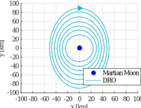
Nowadays, distant retrograde orbit (DRO) attracts consider- able attention from researchers and engineers. DRO is a peri- odic orbit in the circular restricted three-body problem that, in the rotating frame, looks like a large quasi-elliptical retrograde orbit around the secondary body (Fig. 1). DROs are stable over long periods. All the eigenvalues of the monodromy matrix of the DRO equal 1. This indicates that DRO is Lyapunov stable and the relative distance of the spacecraft from the DRO dose not diverge under small perturbations. Thanks to its stability, DRO is an ideal orbit for the spacecraft to collect scientific data and samples.

DRO has been studied in systems with large relative mass such as the Earth-Moon system or Jupiter-Europa system for a long time.

^{1) 2)}

In recent years, DRO has been expected for use in asteroid exploration because DROs around a small mass satellite, such as Phobos or Deimos, show periodic orbits and are convenient for a observation satellite.

³⁾

DRO around the Martian Moon has obtained by numerical calculation such as Newton’s method using the initial value ob- tained from the analytical solution ignoring the gravitational

force exerted on the spacecraft from Martian Moon. For that reason, if the size of DRO is relatively small, the numerical calculation does not converge due to the influence of the grav- ity term, and the closed orbit may not be obtained. Even if a closed orbit can be computed, another problem is possibly time-consuming computation.

In this paper, we analytically study DRO around the Martian moon, not numerically as in the conventional approaches. Par- ticularly, we provide the analytical relations between the ampli- tude ratios and the orbital angular velocities, which are valid for not only planar DROs in the xy plane but also for DROs with vertical component (3D DROs). The outline of the proposed analytical approximation is as follows. First, independent vari- ables in basic equations of the relative motion are approximated by trigonometric functions. Second, basic equations of the rela- tive motion are transformed into a time-independent form using a Fourier series. Since the gravitational force exerted on the spacecraft from the Martian Moon contains plural frequency components, this makes difficult to obtain a Fourier series for the fundamental frequency component. To overcome the diffi- culty and to obtain the analytical relations between the ampli- tude ratios and the orbital angular velocities, we introduce an approximation scheme.

By the analytical expression of this paper, it is possible to

obtain candidates of closed orbits in various conditions without

searching based on numerical calculation. Since the proposed

analytical expression is obtained by an approximation, the re-

sultant trajectory is not necessarily a closed orbit. Even in such

a case, however, a closed orbit can be easily obtained by pro-

viding the resultant trajectory to Newton’s method as an initial

solution.

-100 -80 -60 -40 -20 0 20 40 60 80 100 x [km]

-100 -80 -60 -40 -20 0 20 40 60 80 100

y [km]

Martian Moon DRO

Fig. 1. Typical DROs

2. Modeling 2.1. Hill equation

An asteroid is assumed to move around a primary body based on a two-body problem. By setting a spacecraft position around the asteroid as r = [x, y, z]

^T

in the LVLH coordinates with the origin at the center of mass of the asteroid, the time evolution of the spacecraft is governed by the following equations:

x

^′′

− 2 y

^′

− 3x = − α

r ³ x (1)

y

^′′

+ 2x

^′

= − α

r ³ y (2)

z

^′′

+ z = − α

r ³ z , (3)

where the distance is normalized by dividing by the reference values of 1 AU, and the time is also normalized by dividing the orbital period of the asteroid by 2π. r are given by

r = √

x ² + y ² + z ² . (4) 2.2. Approximation of solution

Consider a planar DRO in the xy plane, the trajectory is ap- proximated as a clockwise elliptical orbit. Then x and y are expressed as follows:

x = a

x

sin( ω

xy

τ ) (5) y= a

_y

cos( ω

xy

τ ) , (6) where ω

xy

is the normalized orbital angular velocity, and in the case of ignoring the asteroid’s gravity, ω

xy

= 1. On the contrary, consider a 3D DRO, z is expressed as follows:

z = a

z

sin( ω

z

τ + ϕ

z

) . (7) If ω

xy

/ω

z

is a rational number, s closed orbit is obtained as 3D DRO. By substituting Eqs. (5)-(7) into Eqs. (1)-(3), the follow- ing equations are obtained:

( −ω ²

xy

+ 2 ξω

xy

− 3 )

sin( ω

xy

τ ) = − f sin( ω

xy

τ ) (8) ( −ξω ²

xy

+ 2 ω

xy

) cos( ω

xy

τ ) = f ξ cos( ω

xy

τ ) (9) ( −ω ²

z

ϵ 1 + ϵ 1

) sin( ω

z

τ + ϕ

z

) = − f ϵ 1 sin( ω

z

τ + ϕ

z

) , (10) where ξ , ϵ

1

and f are given as follows:

ξ = a

_y

a

_x

, ϵ 1 = a

z

a

_y

,

f = α

a ³

_y

( sin

²

(

ωxyτ

)

ξ²

+ cos ² ( ω

xy

τ ) + ϵ ₁ ² sin ² ( ω

z

+ ϕ

z

) )

³₂

. (11)

2.3. New analytical relations between the amplitude ratios and the orbital angular velocities

Here, we derive analytical relations between the amplitude ratios ξ and ϵ

1

, and the orbital angular velocities ω

xy

and ω

z

by comparing the coefficients of trigonometric functions in Eqs.

(8)-(10). Since they are also included in f , let us extract only the fundamental frequency component by expanding f into a Fourier series. Since, however, f contains two frequency com- ponents ω

xy

and ω

z

, this makes di ffi cult to obtain a Fourier coef- ficient for the fundamental frequency component. To overcome the di ffi culty and to obtain the analytical relations between the amplitude ratios and the orbital angular velocities, we introduce an approximation scheme for f . First, we impose the following assumptions:

• Assume ϵ

₁²

≪ 1 and ignore the higher order terms;

• Let ϵ

2

be 1 − ω

z

/ω

xy

and assume |ϵ

2

| ≪ 1; and

• f ≈ f |

_ϵ²_1=0,ϵ2=0

+

_∂ϵ^∂f2 1

_ϵ2

1=0,ϵ2=0

ϵ

₁²

+

_∂ϵ^∂f₂

_ϵ2

1=0,ϵ2=0

ϵ

2

. 1. On the basis of ω

xy

Substituting ω

z

= (1 − ϵ

2

) ω

xy

with Eq. (11), f is expressed as follows:

f ≈ α

a ³

_y

R ³ ( ω

xy

)

  1 − 3 sin ² ( ω

xy

τ + ϕ

z

) 2R ² ( ω

xy

) ϵ 1 ²

  . (12)

2. On the basis of ω

z

Substituting ω

xy

= ω

z

/(1−ϵ

2

) with Eq. (11), f is expressed as follows:

f ≈ α a ³

_y

R ³ ( ω

z

)

[

1 − 3 sin ² ( ω

z

τ + ϕ

z

) 2R ² ( ω

z

) ϵ 1 ²

+ 3 ( ξ ² − 1 )

sin( ω

z

τ ) cos( ω

z

τ ) ω

z

τ ξ ² R ² ( ω

z

) ϵ 2

] , (13)

where R(ω) = √

sin

²

(ωτ)/ξ

²

+ cos

²

(ωτ). The Fourier series of Eq. (8) and Eq. (9) are obtained using Eq. (12), and the following equations are obtained:

ω

xy

π

∫

^2π

ωxy

0

f sin ² ( ω

xy

τ )d τ

= 2 αξ ² π a ³

_y

( 2 g

_ξ

+ h

_ξ

ϵ ₁ ² sin ² ( ϕ

z

) + j

_ξ

+ ϵ ₁ ² cos ² ( ϕ

z

) )

(14) ω

xy

π

∫

^2π

ωxy

0

f sin( ω

xy

τ ) cos( ω

xy

τ )d τ = 2 αξ ²

π a ³

_y

h

_ξ

ϵ 1 ² sin( ϕ

z

) cos( ϕ

z

) (15) ω

xy

π

∫

^2π

ωxy

0

f cos ² ( ω

xy

τ )d τ

= 2 αξ ² π a ³

_y

( 2 f

_ξ

− l

_ξ

ϵ ₁ ² sin ² ( ϕ

z

) + h

_ξ

+ ϵ ² ₁ cos ² ( ϕ

z

) )

, (16) where f

_ξ

, g

ξ

, h

_ξ

, j

_ξ

, l

_ξ

are functions of only ξ and are defined by

f

_ξ

= K

_ξ

− E

_ξ

ξ ² − 1 (17)

g

_ξ

= − K

_ξ

+ ξ ² E

_ξ

ξ ² − 1 (18)

h

_ξ

= ξ ² [2K

_ξ

− ( ξ ² + 1)E

_ξ

]

( ξ ² − 1) ² (19)

j

_ξ

= ξ ² [

( ξ ² − 3)K

_ξ

− 2 ξ ² ( ξ ² − 2)E

_ξ

]

( ξ ² − 1) ² (20)

l

_ξ

= (3 ξ ² − 1)K

_ξ

− 2(2 ξ ² − 1)E

_ξ

( ξ ² − 1) ² . (21)

Here, K

_ξ

, E

_ξ

are defined by the following equations with K (k) and E(k) as complete elliptic integrals of the first kind and the second kind:

K

_ξ

= K

 



√ 1 − 1

ξ ²

 

 , E

_ξ

= E

 



√ 1 − 1

ξ ²

 



K(k) =

∫ 1

0

√ 1 1 − t ² √

1 − k ² t ² dt

E(k) =

∫ 1

0

√ 1 − k ² t ²

√ 1 − t ² dt .

Further, the Fourier series of Eq. (10) is obtained using Eq.

(13), and the following equations are obtained:

ω

z

π

∫

^2π

ωz

0

f sin ² ( ω

z

+ ϕ

z

)d τ

= 2 α π a ³

_y

[ C 1

,

1 + C 1

,

2 ϵ 1 ² + C 1

,

3 ϵ 2

] (22)

C ₁

_,

₁ = 2 ξ ² f

_ξ

− 2( ξ ² − 1)h

_ξ

cos ² ( ϕ

z

) C 1

,

2 = −ξ ² l

_ξ

+ (2m

_ξ

+ n

_ξ

cos ² ( ϕ

z

)) cos ² ( ϕ

z

) C ₁

_,

₃ = 3

2 ξ ³ ( ξ ² − 1) (

k ₃₁ sin ² ( ϕ

z

)

+ 2k ₂₂ sin( ϕ

z

) cos( ϕ

z

) + k ₁₃ cos ² ( ϕ

z

) ) ω

z

π

∫

^2π

ωz

0

f sin( ω

z

+ ϕ

z

) cos( ω

z

+ ϕ

z

)d τ

= α π a ³

_y

[ C 2

,

1 + C 2

,

2 ϵ 1 ² + C 2

,

3 ϵ 2

] (23)

C ₂

_,

₁ = 2( ξ ² − 1)h

_ξ

sin( ϕ

z

) cos( ϕ

z

) C 2

,

2 = − (m

_ξ

+ n

_ξ

cos ² ( ϕ

z

)) sin( ϕ

z

) cos( ϕ

z

) C ₂

_,

₃ = 3 ξ ³ ( ξ ² − 1) (

(k ₃₁ − k ₁₃ ) sin( ϕ

z

) cos( ϕ

z

) + k 22 (cos ² ( ϕ

z

) − sin ² ( ϕ

z

)) )

,

where m

_ξ

, n

_ξ

, k

31

, k

22

, k

13

are functions of only ξ and are defined by

m

_ξ

= ξ ² [

(9 ξ ² − 1)K

_ξ

− (3 ξ ⁴ + 7 ξ ² − 2)E

_ξ

]

( ξ ² − 1) ² (24)

n

_ξ

= ξ ² [

( ξ ⁴ − 18 ξ ² + 1)K

_ξ

− 2( ξ ⁶ − 5 ξ ⁴ − 5 ξ ² + 1)E

_ξ

] ( ξ ² − 1) ²

(25) k 31 =

∫ 2

π

0

u cos ³ u sin u

[ 1 + ( ξ ² − 1) cos ² u ]

⁵₂

du (26)

k ₂₂ =

∫ 2

π

0

u cos ² u sin ² u

[ 1 + ( ξ ² − 1) cos ² u ]

⁵₂

du (27)

k 13 =

∫ 2

π

0

u cos u sin ³ u

[ 1 + ( ξ ² − 1) cos ² u ]

⁵₂

du . (28)

When Eqs. (8)-(10) cannot be represented by a single sinusoidal function depending on the value of ϕ

z

. In this case, it is not expected that a closed orbit exists. On the other hand, when ϕ

z

is an integral multiple of π/2, Eqs. (8)-(10) can be represented only by sin(ω

xy

τ), cos(ω

xy

τ) and sin(ω

z

τ + ϕ

z

), respectively.

Therefor, equations are expressed with these coefficients. Then Eqs. (8)-(10) are reduced to the followings:

1. In the case of ϕ

z

= 0,

−ω ²

xy

+ 2 ξω

xy

− 3 + 2 αξ ²

π a ³

_y

(2 g

_ξ

+ j

_ξ

ϵ ₁ ² ) = 0 (29)

−ξω ²

xy

+ 2 ω

xy

+ 2 αξ ³

π a ³

_y

(2 f

_ξ

+ h

_ξ

ϵ 1 ² ) = 0 (30)

−ω ²

z

+ 1 + 2 αξ ² π a ³

_y

[

2 g

_ξ

+ j

_ξ

ϵ 1 ² + 3

2 ξ ( ξ ² − 1)k 13 ϵ 2

]

= 0 . (31) 2. In the case of ϕ

z

= π/ 2,

−ω ²

xy

+ 2 ξω

xy

− 3 + 2 αξ ²

π a ³

_y

(2 g

_ξ

+ h

_ξ

ϵ ₁ ² ) = 0 (32)

−ξω ²

xy

+ 2 ω

xy

+ 2 αξ ³

π a ³

_y

(2 f

_ξ

− l

_ξ

ϵ 1 ² ) = 0 (33)

−ω ²

z

+ 1 + 2 αξ ² π a ³

_y

[

2 f

_ξ

− l

_ξ

ϵ 1 ² + 3

2 ξ ( ξ ² − 1)k 31 ϵ 2

]

= 0 . (34) By setting ω

z

= (1 −ϵ

2

) ω

xy

, there are five unknowns in these ex- pressions, namely, a

_y

, ω

xy

, ξ, ϵ

1

, and ϵ

2

. Therefore, if we spec- ify two of them, for example a

_y

and ϵ

1

, the remaining unknowns can be determined. It is necessary for the resultant trajectory to form a closed orbit that the ratio of ω

xy

and ω

z

is a rational num- ber. For example, if a trajectory revolves (N + 1) times in the xy plane, while its z-axis component has period N , the following condition must hold:

ω

xy

ω

z

= N + 1

N . (35)

Substituting ω

z

= (1 − ϵ

2

)ω

xy

with Eq. (35), ϵ

2

is expressed as follows:

ϵ 2 = 1

N + 1 . (36)

Actually, a closed orbit when ϕ

z

= 0 is not obtained by numeri- cal calculation in many cases. In the following, we examine the nature of the solution mainly for the case of ϕ

z

= π/2.

By the analytical expression, it is possible to obtain candi-

dates of closed orbits in various conditions without searching

based on numerical calculation. Since the proposed analytical

expression is obtained by an approximation, the resultant tra-

jectory is not necessarily a closed orbit. Even in such a case,

however, a closed orbit can be easily obtained by providing the

resultant trajectory to Newton’s method as an initial solution.

3. Orbital Stability

3.1. Linearization around the equilibrium point

When a 3D DRO is obtained, its stability is analyzed by lin- earizing the equations of motion around the DRO. It can be determined from the eigenvalues of the monodromy matrix by obtaining the solution numerically. On the other hand, in this section, by linearizing the variables around the analytically ob- tained equilibrium point, the eigenvalues of the analytical mon- odromy matrix can be obtained. Thus, it is not necessary to perform numerical calculation,and the stability under various conditions can be easily analyzed. The equilibrium point ˜ r is given by:

r ˜ =

 



¯ x y ¯

¯ z

 

 =

 



a_y

ξ

sin( ω

xy

τ ) a

_y

cos( ω

xy

τ ) ϵ 1 a

_y

sin( ω

z

τ + ϕ

z

)

 

 . (37)

The equation of motion for the deviation from the equilibrium point, which is denoted by η = r − ˜ r, becomes as follows:

ζ

^′

= (A + δ A) ζ, ζ =

[ η

η

^′

]

(38)

A =

 









0 0 0 1 0 0

0 0 0 0 1 0

0 0 0 0 0 1

3 0 0 0 2 0

0 0 0 − 2 0 0

0 0 − 1 0 0 0

 







 δ A =

[ 0 3

×

3 0 3

×

3

− _˜

_r^α3

( I 3

×

3 − 3ˆ˜ rˆ˜ r

^T

) 0 ₃

_×

₃

]

˜

r = | ˜ r|, ˆ˜ r = ˜ r

˜ r ,

where δA is a perturbation matrix that represents the effects of the gravitational force exerted on the spacecraft from the aster- oid in linearization equations into account.

3.2. State transition matrix

When the gravity effects are expressed by a small linear term, the stability of the system can be determined from the state tran- sition matrix of the linearized equation. Because the state tran- sition matrix is difficult to be obtained directly, it would be cal- culated perturbatively. By regarding δ A as a perturbation term, the state transition matrix Φ including the e ff ects is expressed as follows:

Φ = Φ 0 (I 6

×

6 + δΦ + · · · ) , (39) where Φ

0

and Φ are both linear state transition matrices and satisfy the following expressions:

d

d τ Φ 0 ( τ, 0) = AΦ 0 ( τ, 0) (40) d

d τ Φ ( τ, 0) = ( A + δ A( τ )) Φ 0 ( τ, 0) . (41) Also, δΦ in Eq. (39) is the first order perturbation terms. By substituting Eq. (39) into Eq. (41) and equating the first order terms with respect to δ of both sides, the following equation is obtained:

d

d τ δΦ ( τ, 0) = Φ 0 ( τ, 0) δ A( τ ) Φ 0 (0 , τ ) . (42)

Therefor, the state transition matrix including the first order gravity effects of the asteroid can be approximately obtained by integrating the above equation. The state transition matrix after one cycle under the effects of the gravity force from the aster- oid is expressed as Φ(T, 0), while the deviation caused by the gravity effects is expressed as δΦ(T, 0). The deviation δΦ(T, 0) is calculated by

δΦ (T , 0) =

∫

T

0

Φ 0 ( τ, 0) δA( τ ) Φ 0 (0 , τ )d τ. (43) The integral in Eq. (43) can be calculated using an elliptic inte- gral. Hence, the monodromy matrix Φ(T, 0) is obtained using Eqs. (39), (43):

Φ (T , 0) = Φ 0 (T , 0) [

I 6

×

6 +

∫

_T

0

Φ 0 ( τ, 0) δA( τ ) Φ 0 (0 , τ )d τ ]

. (44) In order to calculate the integral in Eq. (44), it is necessary to multiply Φ

0

(τ, 0) from left and Φ

0

(0, τ) from right. These matrices are expressed as follows:

Φ 0 ( τ, 0) = exp(Aτ ) (45) Φ 0 (0 , τ ) = Φ 0 ( −τ, 0) . (46) 3.3. Stability of closed orbits

The stability of the equilibrium point is determined by check- ing whether Φ(T, 0) has an eigenvalue whose absolute value is larger than 1. T denotes the period of ˜ r, and we consider the pe- riod such that T = 2(N + 1)π/ω

xy

= 2Nπ/ω

z

holds. However, it is difficult to solve Φ(T, 0) analytically because T depends on N and is also different from the period of the asteroid. Therefor, considering ω

xy

≈ ω

z

≈ 1 as in the case of ignoring the grav- ity of the asteroid, δΦ(T, 0) is approximated by δΦ(2π, 0). The motion of the spacecraft in the z direction can be regarded as independent by Eqs. (1)-(3) if the gravity force is small. There- for, we investigate the influence on the stability in the z direc- tion due to deviation in the z direction. The (i, j)th component of Φ(T,0) is denoted as Φ

i,j

. When ϕ

z

= π/2, its components in the z direction are obtained using Eq. (44):

Φ 3

,

3 = 1 (47)

Φ 3

,

6 = 4 αξ ²

a ³

_y

( g

_ξ

+ h

_ξ

ϵ 1 ² ) (48) Φ 6

,

3 = 4 αξ ²

a ³

_y

( − f

_ξ

+ l

_ξ

ϵ 1 ² ) (49) Φ 6

,

6 = 1 . (50) In order to investigate the influence of the amplitude ratio ϵ

1

in the z direction on the stability of the closed orbit, we focus on only the components in the z direction, and examine the ab- solute values of those eigenvalues. Although all components generally interact with each other, the z direction components are relatively independent of the other directions. Thus we sep- arately investigate only the z direction components. The eigen- values can be expressed as follows:

det (

λI 2

×

2 −

[ Φ 3

,

3 Φ 3

,

6

Φ 6

,

3 Φ 6

,

6

])

= 0

= ⇒ λ = 1 ± √

Φ 3

,

6 Φ 6

,

3 . (51)

From the above eigenvalues, the stability in the z direction is concluded as

Φ 3

,

6 Φ 6

,

3 > 0 : unstable . (52) In the case of Φ

3,6

Φ

6,3

> 0, the system has an eigenvalue larger than 1, and the closed orbit is unstable. Expanding Eq. (52) and ignoring the term of ϵ

₁⁴

, the following sufficient condition for the closed orbit to be unstable:

ϵ 1 >

√ f

_ξ

g

_ξ

l

_ξ

g

ξ

− h

_ξ

f

_ξ

. (53) Because the right hand side of the condition in Eq. (53) depends only on ξ, it is independent of other parameters. Furthermore, since ξ is the amplitude ratio of the y direction to the x direction of DRO, it takes a value in 1 < ξ < 2. Figure 2 shows the su ffi cient conditionfor the closed orbit to be unstable. As shown in Fig. 2, the value on the right side of the above equation takes a value of about 0.55 ∼ 0.58 for the variation of ξ.

unstable

Fig. 2. Analytically derived unstable region

4. Numerical Examples

In this section, we first compare trajectory characteristics be- tween the numerical solution and the analytical one obtained from Eqs. (32)-(34). Next, we compare the stability region ob- tained by the instability condition (53), and that computed from the numerical solutions.

4.1. Analytical solutions

When ϕ

z

= π/2, the analytical results of ϵ

2

, ω

xy

and ξ with respect to the values of a

_y

and ϵ

1

are shown in Fig. 3 using Eqs.

(32)-(34). We set the parameters α and a

p

to those of Mars and Deimos, namely,

α = 2 . 8 × 10

⁻

⁹ , a

p

= 23458 [km] .

where a

p

denotes the normalized revolution radius of Deimos by the relative distance. Since ϵ

2

is always positive, it is implied that ω

z

is smaller than ω

xy

. Therefore, when the number of turns in the z direction is smaller than the number of turns in the xy plane, there can be a closed orbit. Although ϵ

2

, ω

xy

and ξ change depending on ϵ

1

, the variations are small when ϵ

1

is between 0 and 0.6. As a

_y

becomes smaller, the value of ω

xy

becomes larger.

4.2. Comparisons of numerical and analytical solutions The proposed analytical solution with Newton’s method en- ables us to easily obtain a closed orbit. We obtain a numerical solution for each combination of N = 4, 11, ϵ

1

= 0.1, 0.3 and ϕ

z

= π/2. The results obtained are shown in Fig. 4, where the relative distance is indicated by the actual distance. The com- parisons of the numerical and analytical solutions of ϵ

2

, ω

xy

, ξ are shown in Figs. 5 and 6. These figures show that the pro- posed analytical solutions have good consistency with numeri- cal solutions. Therefore, it can be concluded that the proposed analytical equations (32)-(34) properly represent the closed or- bit behavior.

4.3. Orbital Stability

In this subsection, the stability of the closed orbit is investi- gated. The stability of the numerical solution can be examined from the eigenvalues of the monodromy matrix numerically ob- tained as described above. We compare this with the analyti- cally derived instability condition in Eq. (53). The results are shown in Fig. 7. In this figure, the instability condition is indi- cated by a blue line, and the region above this blue line exhibits the analytical result of the unstable region. The result of numer- ical solution is indicated by a circle, and the green indicates that the absolute value of the eigenvalue of the monodromy matrixis is 1.5 or less, which is not clearly unstable. On the one hand, the red indicates that it is greater than 1.5, which is clearly unstable.

Some discrepancies are observed, where the analytical condi- tion implies instability, though numerical solution shows that it is stable, and vice versa. Possible reasons for those discrepan- cies are that the analytical solution considers only the stability in the z direction, and that derivation of the present analytical solution requires several approximations. A more exact stabil- ity condition considering the influence of the xy plane motion will be a future work.

5. Conclusions

In this paper, the periodic orbits of the spacecraft around the asteroid has been considered. In particular, we have studied the trajectory characteristics and stability of 3D-DRO around Deimos.

Basic equations of the relative motion are transformed into a time-independent form by using a Fourier series. Then, to ob- tain the analytical relations between the amplitude ratios and the orbital angular velocities, we have introduced an approximation scheme. It can be concluded that the analytical equations prop- erly represent the closed orbit behavior.

A periodic orbit to be analyzed is linearized around the equi- librium point, and the stability of the system is concluded by the eigenvalues of the state transition matrix. We have newly provided a su ffi cient condition for a closed orbit to be unstable.

Using the analytical expression of this paper, it is possible to obtain candidates of closed orbits in various conditions without searching based on numerical calculation.

References

1) Ani N.Hirani, Ryan P.Russell,”Approximations of Distant Ret- rograde Orbits for Mis- sion Design” American Astronomical Society,06-116,2006

2) Try Lam, Gregory J. Whi ff en,”Exploration of Distant Retro-

Grade Orbits Around Europa” American Astronomical Society,05- 110,2005

3) Mark Wallace, Je ff rey Parker, Nathan Strange, and Daniel Grebow : Orbital Operations for Phobos and Deimos Exploration, AIAA / AAS Astrodynamics Specialist Conference, Guidance, Navigation, and Control and Co-located Conferences

0 0.002 0.004 0.006 0.008 0.01 ay

0 0.1 0.2 0.3 0.4

eps2

eps1 = 0 eps1 = 0.3 eps1 = 0.6

(a)-1 ϵ

2

0 0.002 0.004 0.006 0.008 0.01 ay

1 1.5 2 2.5 3

omegaxy

eps1 = 0 eps1 = 0.3 eps1 = 0.6

(a)-2 ω

xy

0 0.002 0.004 0.006 0.008 0.01 ay

1 1.2 1.4 1.6 1.8 2

xi

eps1 = 0 eps1 = 0.3 eps1 = 0.6

(b)-1 ξ

Fig. 3. analytical results of ϵ

2

, ω

xy

, and ξ w.r.t. a

_y

and ϵ

1

( ϕ

z

= π/ 2)

-15 -10 200 -5 0

100 60

z [km]

5

40 y [km]

10

0 20

x [km]

15

-100 -200 -60 -40 -20 0

(a)-1 N = 11, ϵ

1

= 0.1

-40 200 -20 0

100 60

z [km]

40 20

y [km]

0 20

x [km]

40

-100 -200 -60 -40 -20 0

(a)-2 N = 11, ϵ

1

= 0.3

-6 -4 100 -2 0

50 40

z [km]

2

y [km]

20 4

0

x [km]

6

-50 -20 0

-100 -40 (b)-1 N = 4, ϵ

1

= 0.1

-30 -20 100 -10 0

50 40

z [km]

10

y [km]

20 20

0

x [km]

30

-50 -20 0

-100 -40 (b)-2 N = 4, ϵ

1

= 0.3

Fig. 4. The resultant closed orbit for each combination of N = 4, 11,

and ϵ

1

= 0 . 1 , 0 . 3 . ( ϕ

z

= π/ 2)

0 0.002 0.004 0.006 0.008 0.01 ay

0 0.05 0.1 0.15 0.2 0.25 0.3 0.35

eps2

analytical numerical

(a)-1 ϵ

2

0 0.002 0.004 0.006 0.008 0.01 ay

1 1.2 1.4 1.6 1.8 2

omegaxy

analytical numerical

(b)-1 ω

xy

0 0.002 0.004 0.006 0.008 0.01 ay

1.3 1.4 1.5 1.6 1.7 1.8 1.9 2

xi

analytical numerical

(c)-1 ξ

Fig. 5. Comparisons between numerical and analytical solutions of ϵ

2

, ω

xy

and ξ ( ϵ

1

= 0 . 1 , ϕ

z

= π/ 2)

0 0.002 0.004 0.006 0.008 0.01 ay

0 0.05 0.1 0.15 0.2 0.25 0.3 0.35

eps2

analytical numerical

(a)-2 ϵ

2

0 0.002 0.004 0.006 0.008 0.01 ay

1 1.2 1.4 1.6 1.8 2

omegaxy

analytical numerical

(b)-2 ω

xy

0 0.002 0.004 0.006 0.008 0.01 ay

1.3 1.4 1.5 1.6 1.7 1.8 1.9 2

xi

analytical numerical

(c)-2 ξ

Fig. 6. Comparisons between numerical and analytical solutions of ϵ

2

, ω

xy

and ξ ( ϵ

1

= 0 . 3 , ϕ

z

= π/ 2)

1.4 1.5 1.6 1.7 1.8 1.9 2

xi 0

0.1 0.2 0.3 0.4 0.5 0.6

eps1 stable

unstable analytical

Fig. 7. Comparison of numerical stability results and the analytical instability condition