Secondary flows of viscoelastic fluids in serpentine microchannels

(1)

Secondary flows of viscoelastic fluids in serpentine microchannels

Author Lucie Ducloue, Laura Casanellas, Simon J.

Haward, Robert J. Poole, Manuel A. Alves, Sandra Lerouge, Amy Q. Shen, Anke Lindner journal or

publication title

Microfluidics and Nanofluidics

volume 23

number 33

year 2019‑02‑05

Publisher Springer Berlin Heidelberg

Rights (C) 2019 Springer‑Verlag GmbH Germany, part of Springer Nature

This is a post‑peer‑review, pre‑copyedit version of an article published in

Microfluidics and Nanofluidics. The final authenticated version is available online at:

http://dx.doi.org/10.1007/s10404‑019‑2195‑0 Author's flag author

URL http://id.nii.ac.jp/1394/00000966/

doi: info:doi/10.1007/s10404-019-2195-0

(2)

UN CORRECTED PR

OOF

Vol.:(0123456789)

1 3

Microfluidics and Nanofluidics _#####################_

https://doi.org/10.1007/s10404-019-2195-0 RESEARCH PAPER

Secondary flows of viscoelastic fluids in serpentine microchannels

Lucie Ducloué¹ · Laura Casanellas^1,2 · Simon J. Haward³ · Robert J. Poole⁴ · Manuel A. Alves⁵ · Sandra Lerouge⁶ · Amy Q. Shen³ · Anke Lindner¹

Received: 25 October 2018 / Accepted: 16 January 2019

Abstract

Secondary flows are ubiquitous in channel flows, where small velocity components perpendicular to the main velocity appear due to the complexity of the channel geometry and/or that of the flow itself such as from inertial or non-Newtonian effects.

We investigate here the inertialess secondary flow of viscoelastic fluids in curved microchannels of rectangular cross-section and constant but alternating curvature: the so-called “serpentine channel” geometry. Numerical calculations (Poole et al. J Non-Newton Fluid Mech 201:10–16, 2013) have shown that in this geometry, in the absence of elastic instabilities, a steady secondary flow develops that takes the shape of two counter-rotating vortices in the plane of the channel cross-section. We present the first experimental visualization evidence and characterization of these steady secondary flows, using a complementarity of μPIV in the plane of the channel, and confocal visualisation of dye-stream transport in the cross-sectional plane. We show that the measured streamlines and the relative velocity magnitude of the secondary flows are in qualitative agreement with the numerical results. In addition to our techniques being broadly applicable to the characterisation of three-dimensional flow structures in microchannels, our results are important for understanding the onset of instability in serpentine viscoelastic flows.

Keywords Polymer solutions · Non-Newtonian fluids · Vortices · Confocal microscopy · Particle image velocimetry

1 Introduction

Three-dimensional velocity fields are widespread in channel and pipe flows, where the geometry of the duct can combine with the properties of the base primary flow (i.e. the flow in the streamwise direction) to trigger a weak current with velocity components perpendicular to the streamwise direction. Therefore, the ability to measure, and understand, the velocity field in all three directions of such flows is of general importance. In microfluidic flows, however, the flow- field in the streamwise direction is often the only component characterised, because of optical access limitations and due to the fact that the absolute value of the other velocity components are typically very small (Tabeling 2005). Despite their small magnitude, such secondary flows are often ulti- mately responsible for enhanced mixing (above that due to diffusion alone) of mass and heat which is a frequent aim of various microfluidic devices (Lee et al. 2011; Mitchell 2001;

Stroock et al. 2002; Amini et al. 2013; Hardt et al. 2005;

Kockmann et al. 2003). Secondary flows also have important implications in particle focussing (Del Giudice et al. 2015;

* Anke Lindner [email protected]

1 Laboratoire de Physique et Mécanique des Milieux Hétérogènes, UMR 7636, CNRS, ESPCI Paris, PSL Research University, Université Paris Diderot, Sorbonne Université, Paris 75005, France

2 Present Address: Laboratoire Charles Coulomb UMR 5221 CNRS-UM, Université de Montpellier, Place Eugène Bataillon, 34095 Montpellier Cedex 5, France

3 Okinawa Institute of Science and Technology Graduate University, Onna, Okinawa 904-0495, Japan

4 School of Engineering, University of Liverpool, Brownlow Street, Liverpool L69 3GH, UK

5 Departamento de Engenharia Química, Centro de Estudos de Fenómenos de Transporte, Faculdade de Engenharia da Universidade do Porto, Rua Doutor Roberto Frias, 4200-465 Porto, Portugal

6 Laboratoire Matière et Systèmes Complexes, CNRS UMR 75057-Université Paris Diderot, 10 rue Alice Domond et Léonie Duquet, 75205 Paris Cedex, France

AQ1 1

2

3 4

5 6

7 8 9 10 11 12 13 14 15 16 17 18 19

20

21

22 23 24 25 26 27 28 29 30 31 32 33 34 35 36 37 38 39 40 A1

A2

A3 A4 A5 A6 A7 A8 A9 A10 A11 A12 A13 A14 A15 A16 A17 A18 A19 A20

(3)

UN CORRECTED PR

OOF

Di Carlo et al. 2007) where they may either be exploited or act as a hindrance.

Secondary flows in microfluidic systems may be driven by the complexity of the channel geometry only: for the creeping flow of a Newtonian fluid, Lauga et al. (2004) have shown that a secondary flow must develop if the channel has both varying cross-section and streamwise curvature.

Changes in the streamwise curvature of channels with constant cross-section have also been shown to give rise to a secondary flow around the bend (Guglielmini et al. 2011;

Sznitman et al. 2012). More complex geometries have been designed to obtain chaotic micromixers, in which secondary flows are triggered and expose volumes of fluid to a repeated sequence of rotational and extensional local flows (Ottino 1989; Stroock et al. 2002; Amini et al. 2013).

Complexity in the equations of fluid motion is another driving mechanism for secondary flows: although usually not dominant at the microscale, inertia can play a role in microfluidic systems (Di Carlo 2009; Amini et al. 2014).

Combined with the flow geometry, it drives secondary flows such as the well-known “Dean” vortices (Dean 1927, 1928) observed in curved channels and pipes, or the steady vortical structure of the “engulfment” regime in T-junction mixers (Kockmann et al. 2003; Fani et al. 2013). In the absence of inertia, viscoelasticity is another source of fluid dynamic complexity: viscoelastic analogues of the Dean vortices are formed, in the creeping-flow regime, by the coupling of the first normal-stress difference with streamline curvature (Robertson and Muller 1996; Fan et al. 2001; Poole et al. 2013; Bohr et al. 2018). Note that second-normal stress differences in viscoelastic fluids may also drive an inertialess secondary motion in ducts of non-axisymmetric cross- section, but this flow is typically much weaker (Gervang and Larsen 1991; Debbaut et al. 1997; Xue et al. 1995). We emphasise that in listing those potential sources of secondary flow we are not attempting to be exhaustive, but sim- ply to illustrate that they may occur under many different scenarios.

We focus here on the viscoelastic secondary flow driven by streamline curvature. This steady secondary flow is always present in the steady flow of viscoelastic fluids in curved geometries, and pertains at all flow rates until a critical flow rate is reached at which the flow becomes time-dependent due to a well-known purely elastic instability (Groisman and Steinberg 2000; Arratia et al. 2006;

Afik and Steinberg 2017; Souliès et al. 2017). Characterising this secondary flow is thus essential to the knowledge of the three-dimensional base flow from which the elastic instability develops: its structure may interact with the onset of the instability, as hypothesised to explain the partially unac- counted for stabilisation of shear-thinning viscoelastic flow in curved microchannels (Casanellas et al. 2016). It is also important for mixing and particle focusing applications that

rely on viscoelastic fluids (Groisman and Steinberg 2000;

Del Giudice et al. 2015).

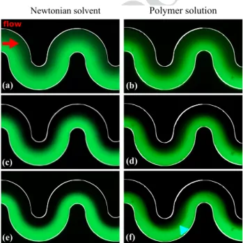
Evidence for such secondary flows is readily observable in simple visualisation experiments. By way of example, in Fig. 1 we show a classical experiment for the visualisation of mixing efficiency in a serpentine microchannel (Grois- man and Steinberg 2000): two streams of the same fluid, one of them dyed with fluorescein, are co-injected into the serpentine micromixer. When a Newtonian fluid is injected, mixing is achieved by diffusion alone, which broadens the interface. With increasing flow rate, the residence time decreases, and so does the width of the interface. When a

Polymer solution Newtonian solvent

(a) (b)

(c) (d)

(e) (f)

flow

Fig. 1 Visualisation of mixing in a serpentine microchannel (the channel edges are highlighted in white): two streams of fluid are co- injected in a Y-junction, one of them being fluorescently labelled.

Data for a viscoelastic polymer solution are displayed on the right- hand side, while data for the Newtonian solvent (a mixture of water and glycerol at 75–25 wt%) (The small fluorescein molecule diffuses almost freely in the polymer network and thus probes a local viscosity that is lower than the shear viscosity of the polymer solution as measured with a rheometer. The same behaviour has been quantified in solutions of (hydroxypropyl) cellulose (Mustafa et al. 1993), dextran (Furukawa et al. 1991) and polyethylene glycol (Holyst et al.

2009). For this reason, we use the solvent of the polymer solution as a Newtonian reference fluid. The slightly lower diffusion in the polymeric solution shows that the contribution from the polymer to the local viscosity, albeit small, is not entirely negligible.) are shown on the left-hand side. The flow rate increases from 2 μl/min (top row) to 6 μl/min (middle row) and 12 μl/min (bottom row). At low flow rates (a, b) the interface between the two streams is broadened in both cases by the strong diffusion of the dye. At larger flow rates (c and d), the interface sharpens all along the channel due to the decreas- ing residence time. Further increase of the flow rate (e and f) leads to further sharpening of the interface for the Newtonian flow (e), but an additional spatially varying “blur” develops in the viscoelastic flow (f), blue triangular arrow

41 42 43 44 45 46 47 48 49 50 51 52 53 54 55 56 57 58 59 60 61 62 63 64 65 66 67 68 69 70 71 72 73 74 75 76 77 78 79 80 81 82 83 84 85 86 87 88 89 90 91 92 93

94 95 96 97 98 99 100 101 102 103 104 105

(4)

UN CORRECTED PR

OOF

1 3

Page 3 of 10 _####_

viscoelastic fluid is used, the evolution of the width of the interface with increasing flow rate is very different. At small flow rates a very broad interface is again observed, which initially sharpens when the flow rate is increased. When the flow rate is further increased, however, the interface locally widens again. This effect cannot be attributed to diffusion, which becomes less important with increasing flow rate (thus decreasing residence times). In addition, an asymmetry can be observed with the interface being significantly wider towards the end of each loop and a sharpening of the interface at the beginning of each new loop. This observation can only be explained with an underlying three dimensional flow structure that reverses direction in between consecutive loops. Previous numerical simulations (Poole et al. 2013) have shown the occurrence of a steady secondary flow in this serpentine channel geometry for dilute viscoelastic liquids.

One of the aims of this work is to demonstrate and quantify the occurrence of this secondary flow experimentally by direct measurement. More generally, we show how different experimental methods can be used to determine quantitative information of generic secondary flows in micro-devices.

Being typically very weak (on the order of a few per- cent of the bulk primary velocity), secondary flows are hard to resolve even in macro-sized classical fluid mechanics experiments (Gervang and Larsen 1991). Thus it is not sur- prising that such flows have been little characterised at the microscale. A number of recent experimental approaches may alleviate this issue, in particular the holographic microparticle tracking velocimetry ( μPTV) technique (Salipante et al. 2017), confocal microparticle image velocimetry (confocal μPIV) (Li et al. 2016) or using standard particle image velocimetry in conjunction with a channel design and mate- rial that allow for microscope observation in several perpendicular planes (Burshtein et al. 2017).

Here, we will characterise experimentally the three- dimensional structure of the flow with supporting numerical simulations that match the geometrical conditions. Our aim is to use a complementarity of μPIV , confocal microscopy and insight gleaned from simulation to quantify the secondary flow and confirm its vortical structure and sense of rotation. Our techniques are very generic and thus broadly applicable to the characterisation of three-dimensional flow structures in microchannels.

2 Experimental and numerical methods

2.1 Working fluids and rheological characterisation Model viscoelastic fluids were prepared by dissolving polyethylene oxide (PEO, from Sigma Aldrich) with a molecular weight of M_W=4×10⁶ g/mol in a water/glycerol (75–25%

in weight) solution. The PEO was supplied from the same

batch as used in Casanellas et al. (2016). The solvent viscosity at T=21^◦ C is 𝜂_s=2.1 mPa s (data not shown). The polymer concentration was fixed to c=500 ppm (w/w).

The total viscosity of the resulting solution at T=21^◦ C is 𝜂=3.8 mPa s giving a solvent-to-total viscosity ratio 𝛽 = 0.55. The overlap concentration for this polymer in water is c^∗ ≃550 ppm (Casanellas et al. 2016). Although this solution is close to the semi-dilute limit, we confirmed that shear-thinning effects, of both the shear viscosity and the first normal-stress difference, are essentially negligible [see e.g. Casanellas et al. (2016)].

2.2 Microfluidic geometry

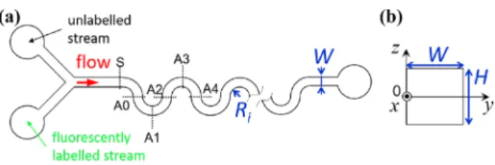
We tested the polymer solution in serpentine microchannels consisting of nine half loops. A sketch of the channel is shown in Fig. 2. We note that, in this channel geometry, the absolute value of the curvature is constant along the channel but the sign of the curvature changes from positive to nega- tive between consecutive half-loops. This change of sign is not required for the development of the viscoelastic secondary flow, but is a feature of our two-dimensional geometry which conveniently allows for the study of several consecutive loops at a constant radius of curvature. Numerical simulations of the creeping flow of Newtonian fluids in bent microchannels show that this change in curvature is expected to trigger a local secondary flow where subsequent half- loops reconnect, but this flow quickly decays in the regions of constant curvature (Guglielmini et al. 2011), where our velocity measurements were made. Most of our results were obtained on a channel of nearly square cross-section, with a width W =110±3 μ m, height H=99±1 μ m and an inner radius of curvature (measured at the inner wall of the channel) R_i=40±1 μ m. Additional channels of comparable cross-sectional dimensions but larger radii of curvature were used for comparison.

The microchannels were fabricated in polydimethyl- siloxane (PDMS), using standard soft-lithography

Fig. 2 Schematic of the microfluidic geometry used: a top view and b cross-sectional view displaying the choice of axes. x is the primary flow velocity direction, y is the wall-normal direction (where the origin is taken at the inner edge of each loop), and z is the spanwise (vertical) direction. Therefore, the x, y, z coordinate system we con- sider is not fixed in space but advected with the flow. The location of the dyed stream used for confocal visualisation is also indicated AQ2

106 107 108 109 110 111 112 113 114 115 116 117 118 119 120 121 122 123 124 125 126 127 128 129 130 131 132 133 134 135 136 137 138 139 140 141 142 143 144 145 146 147 148

149

150

151 152 153 154

155 156 157 158 159 160 161 162 163 164 165

166

167 168 169 170 171 172 173 174 175 176 177 178 179 180 181 182 183 184 185 186 187 188 189 190

(5)

UN CORRECTED PR

OOF

microfabrication methods (Tabeling 2005), and mounted on a glass coverslip. The fluid was injected into the channel via two inlets using two glass syringes (Hamilton, 500 μ l each) that were connected to a high-precision syringe pump (Nemesys, from Cetoni GmbH). The experimental protocol consisted of stepped ramps of increasing flow rate from 2 μ l/min up to a maximum of 20 μl/min, with a flow rate step of 2 μl/min. The resolution of the applied flow rate was con- trolled at a precision of ± 0.2 μl/min, as confirmed indepen- dently using a flow sensor (Flow unit S, from Fluigent, at low flow rates and SLI-0430 Liquid flow meter, from Sen- sirion for Q≥6 μl/min). The step duration was set to 120 s, and the measurements performed over the last 60 s, which we confirm was long enough to ensure flow steadiness and the decay of any initial transient regime. Experiments were continued until the onset of the purely-elastic instability where the flow became time-dependent. For the R_i=40 μ m channel this occurred at 14 μl/min which we define as Q_insta. At the onset of flow instability the Reynolds number ( Re=𝜌UW∕𝜂 , where 𝜌 is the fluid density and U the mean velocity) is small in all experiments, being at most 0.6.

Therefore, in our microfluidic flow experiments inertial effects can be disregarded.

2.3 Micro‑particle image velocimetry

Quantitative two-dimensional measurements of the flow field were made in the xy-centreplane ( z=0 plane) of the serpentine device (Fig. 2) using a micro-particle image velocimetry ( μPIV ) system (TSI Inc., MN) (Meinhart et al. 2000; Were- ley and Meinhart 2005). For this purpose, no fluorescent dye was used but the test fluid was seeded with 0.02 wt%

fluorescent particles (Fluoro-Max, red fluorescent micro- spheres, Thermo Scientific) of diameter d_p=0.52 μ m with peak excitation and emission wavelengths of 542 nm and 612 nm, respectively. The microfluidic device was mounted on the stage of an inverted microscope (Nikon Eclipse Ti), equipped with a 20× magnification lens (Nikon, NA=0.45 ).

With this combination of particle size and objective lens, the measurement depth over which particles contribute to the determination of the velocity field was 𝛿z_m ≈13 μm (Mein- hart et al. 2000), which is approximately 13% of the channel depth.

The μPIV system was equipped with a 1280×800 pixel high speed CMOS camera (Phantom MIRO, Vision Research), which operated in frame-straddling mode and was synchronized with a dual-pulsed Nd:YLF laser light source with a wavelength of 527 nm (Terra PIV, Continuum Inc., CA). The laser illuminated the fluid with pulses of duration 𝛿t<10 ns, thus exciting the fluorescent particles, which emitted at a longer wavelength. Reflected laser light was filtered out by a G-2A epifluorescent filter so that only the light emitted by the fluorescent particles was detected

by the CMOS imaging sensor array. Images were captured in pairs (one image for each laser pulse), where the time between pulses 𝛥t was set such that the average particle displacement between the two images in each pair was around 4 pixels. Insight 4G software (TSI Inc.) was used to cross- correlate image pairs using a standard μPIV algorithm and recursive Nyquist criterion. The final interrogation area of 16 × 16 pixels provided velocity vector spaced on a square grid of 6.4 × 6.4 μ m in x and y. The velocity vector fields were ensemble-averaged over 50 image pairs.

2.4 Confocal microscopy

Vertical images of the cross-section of the channel (in yz planes) were obtained by confocal microscopy imaging using dyed stream visualisation (as illustrated in the xy plane in Fig. 1). z-stacks of two-dimensional images of size 1024× 1024 pixels in xy planes were acquired at a rate of 6 fps using a laser line-scanning confocal fluorescence microscope (LSM 5 Live, Zeiss), with a 40× water immersion objective lens (1.20 NA). The voxel size was 0.16 × 0.16 × 0.45 μ m in the x−y−z direction.

2.5 Viscoelastic constitutive equation, numerical method and structure of predicted secondary flow

The three-dimensional numerical simulations assume isothermal flow of an incompressible viscoelastic fluid described by the upper-convected Maxwell (UCM) model (Oldroyd 1950) in a channel of matched dimensions to those used in the experiments. The equations that need to be solved are those of mass conservation,

and the momentum balance,

assuming creeping-flow conditions (i.e. the inertial terms are exactly zero), where u is the velocity vector with Cartesian components ( u_x , u_y , u_z ), and p is the pressure. For the UCM model the evolution equation for the polymeric extra-stress tensor, 𝜏 , is

where 𝝉₍₁₎ represents the upper-convected derivative of 𝝉 and 𝜂 the constant polymeric contribution to the viscosity of the fluid, respectively.

Although the UCM model exhibits an unbounded steady- state extensional viscosity above a critical strain rate (1/2𝜆 ), in shear-dominated serpentine channel geometries such model deficiencies are unimportant and it is arguably the simplest differential constitutive equation which can capture (1)

∇⋅𝐮=0,

(2)

−∇p+ ∇⋅𝜏=𝟎,

(3) 𝝉+𝜆𝝉₍₁₎=𝜂 ̇𝜸,

191 192 193 194 195 196 197 198 199 200 201 202 203 204 205 206 207 208 209 210 211 212 213

214

215 216 217 218 219 220 221 222 223 224 225 226 227 228 229 230 231 232 233 234 235 236 237 238 239 240 241

242 243 244 245 246 247 248 249 250 251

252

253 254 255 256 257 258 259 260 261

262 263 264

265 266 267 268 269 270 271

272 273

274 275 276 277 278 279

280 281 282 283 284 285 286 287

(6)

UN CORRECTED PR

OOF

1 3

Page 5 of 10 _####_

many aspects of highly-elastic flows. Many more complex models [e.g. the FENE-P, Giesekus and Phan–Thien–Tanner models, see e.g. Bird et al. (1987)], simplify to the UCM model in certain parameter limits and thus its general- ity makes it an ideal candidate for fundamental studies of viscoelastic fluid flow behaviour. The governing equations were solved using a finite-volume numerical method, based on the logarithm transformation of the conformation tensor. Additional details about the numerical method can be found in Afonso et al. (2009, 2011) and in other previous studies [e.g. Alves et al. (2003a, b)]. For low Deborah numbers De=𝜆U∕R_i (with 𝜆 the relaxation time of the fluid, U the mean velocity and R_i the inner radius of curvature), the numerical solution converges to a steady solution, which was assumed to occur when the L¹ norm of the residuals of all variables reached a tolerance of 10⁻⁶ . Beyond a critical Deborah number, a time-dependent purely-elastic instability occurs. The numerical results in the current paper are restricted to Deborah numbers below the occurrence of this purely-elastic instability, thus the flow remains steady in all simulations.

The structure and strength of viscoelastic secondary flows in a serpentine geometry have been investigated in detail by Poole et al. (2013). The main results of this study are recalled below, and lay the foundations for the simulations that we carry out here, which are focused on the geometry of the experimental system we used. The projected streamlines in the yz plane of the computed secondary flow are shown in Fig. 3a. The flow takes the shape of a pair of counter- rotating vortices in the cross-sectional plane of the channel.

It is driven by the hoop stress, which drives the fluid towards the inner side of the bend close to the top and bottom walls (where the shear rate and thus the first normal stress difference are larger, as illustrated in Fig. 3b). The fluid is then carried back towards the outer edge of the bend at the centreplane ( z=0 ). Although the driving mechanism is different, the resulting qualitative features of this elasticity- driven secondary flow are thus similar to the inertia-driven Dean vortices (Dean 1928). The strength of the viscoelastic secondary flow increases with the elastic contribution to the flow (increasing De) and the curvature of the channel.

Poole et al. (2013) have shown that far from the onset of the purely elastic instabilities, the magnitude of the secondary flow, as quantified by the maximum spanwise velocity u_z,max , scales linearly with De (see Fig. 3c). The structure of the flow has been shown to remain identical for aspect ratios W / H varying from 1 up to 4; accordingly, the scaling for u_z,max with De is not modified by the aspect ratio of the channel. The scaling of the secondary flow strength with the solvent viscosity contribution has also been assessed (Poole et al. 2013), and can be expressed as an effective Deborah number De_eff= (1−𝛽)De where 𝛽 is the ratio of the solvent

viscosity to the total (solvent + polymeric) viscosity. In the UCM model, De_eff=De.

The precise experimental determination of the relaxation time of the fluid is difficult for dilute polymer solutions so that the determination of De for our experimental data is challenging. However, we can use the onset of the purely elastic instability as a reference point to match the Deborah numbers in our numerical and experimental data. For a given serpentine geometry, the flow becomes unstable beyond a critical flow speed, usually expressed in terms of a critical Weissenberg number to quantify the importance of the elastic contribution to the flow:

Wi_insta(R_i) =𝜆U_insta∕W (with Wi=De×R_i∕W the Weis- senberg number) (Zilz et al. 2012). For a given channel geometry Wi∕Wi_insta=De∕De_insta=Q∕Q_insta . Therefore, to enable quantitative comparison between experimental and numerical results, all the results for the channel geometry described above will be presented in terms of the reduced quantity De^∗=De∕De_insta=Q∕Q_insta , with De_insta≈1.24 from the numerical results for the experimental geometry we used ( R_i∕W=0.36 ). De^∗ is independent of 𝛽 and, therefore, the solvent viscosity does not need to be taken into account in the present numerical simulations.

(a)

0 0.1 0.2 0.3 0.4 0.5 0.6

De 0

0.02 0.04 0.06 0.08

uz,max

W/H = 1, R/W = 1 W/H = 2, R/W = 1 W/H = 1, R/W = 3 W/H = 1, R/W = 5 W/H = 1, R/W = 7

(c)

10 20 30 40 50 60 70 80 90 100 110

(b)

/U

Fig. 3 a Numerically predicted structure of the secondary flow:

two counter-rotating vortices develop in the cross-sectional plane of the channel. b Contour plot of the first normal stress difference ( N1∕(𝜂U∕W) ), in the cross-section of the channel ( De=0.5 , W∕H=W∕R=1 ): the strong positive and asymmetric normal stress difference at the top and bottom wall drives the secondary flow. c Numerically calculated scaling of the strength of the secondary flow:

the maximum spanwise velocity scales linearly with De over a wide range of aspect ratio and radius of curvature parameters [adapted from Poole et al. (2013)]

288 289 290 291 292 293 294 295 296 297 298 299 300 301 302 303 304 305 306 307 308 309 310 311 312 313 314 315 316 317 318 319 320 321 322 323 324 325 326 327 328 329 330 331 332 333 334 335 336 337 338 339

340 341 342 343 344 345 346 347 348 349 350 351 352 353 354 355 356 357 358 359 360 361 362

(7)

UN CORRECTED PR

OOF

3 Results

3.1 Flow measurement in the plane of the channel using μPIV

In this section, we show that classical μPIV measurements in the xy centreplane provide significant evidence of the existence of a secondary flow. In this symmetry plane, u_z=0 so that the velocity field is fully characterised by the 2D PIV.

In Fig. 4 we show streamlines constructed from the measured velocity field along the first half loop (i.e. from A0 to A2 as shown in Fig. 2). The blue dashed line highlights the Newtonian result which can be seen to travel in approximate concentric semicircles around the bend. The red lines indi- cate the streamlines of the polymeric solution, which, at low Deborah number, can be seen to match the Newtonian ones very closely. In contrast, with increasing De^∗ (increasing flow rate) there is a marked deviation of the streamlines for the viscoelastic fluid away from the inner bend towards the outer, in good agreement with the sense of the secondary flow predicted by the numerical simulations (Poole et al.

2013) and as discussed above and shown in Fig. 3. These streamline patterns thus provide our first piece of qualitative evidence for the existence of an elastic secondary flow.

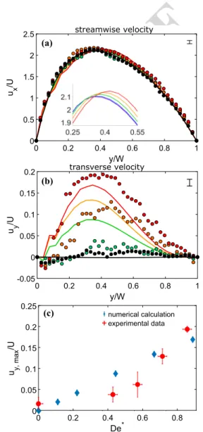
To support these qualitative streamline observations in a more quantitative sense, in Fig. 5 we plot the velocity components around location A1. The primary and wall- normal components of both the experimentally deter- mined (symbols) and the numerically computed (full lines) velocity fields have been averaged over an angular sector of 10^◦ upstream and downstream of A1. y describes as usual the wall-normal direction, and x the primary velocity direction: the primary velocity component is u_x

Fig. 4 Red lines: experimental flow streamlines in the channel centreplane, for increasing values of flow elasticity. For comparison, the streamlines for a Newtonian solution of the same viscosity are shown with a blue dashed line: a clear deviation of the streamlines towards the outer edge of the bend occurs in viscoelastic flow

0 0.05 0.1 0.15 0.2 0.25

u y, max/U

numerical calculation experimental data

(c)(c)

0 0.2 0.4 0.6 0.8

De^*

numerical calculation experimental data

(c)

0 0.2 0.4 0.6 0.8 1

y/W -0.05

0 0.05 0.1 0.15 0.2

u y/U (b)

transverse velocity

0 0.2 0.4 0.6 0.8 1

y/W 0

0.5 1 1.5 2 2.5

u x/U

(a)

streamwise velocity

Fig. 5 Experimental (bullets) and numerical (full lines) velocity plots at location A1 (see Fig. 2) for the primary (a) and wall-normal velocity (b), for increasing values of De^∗ (black bullet Newtonian fluid, green bullet 0.43, orange bullet 0.71, red bullet 0.86 and black full line 0, pink full line 0.11, blue full line 0.22, green full line 0.44, orange full line 0.67, red full line 0.89). For easier comparison, only select De^∗ values are shown in b. The zero y location is taken at the inner edge of the bend, with the geometry being that described in Sect. 2.2: Ri∕W=0.36 . The peak streamwise velocity shifts with De, as is more visible in the inset of a. The scale bar in the top right corner indicates the magnitude of the error on the experimental data. c Scaling for the maximum wall-normal velocity with De^∗

AQ3 363

364 365

366 367 368 369 370 371 372 373 374 375 376 377 378 379 380 381 382 383 384

385 386 387 388 389 390 391 392 393

(8)

UN CORRECTED PR

OOF

1 3

Page 7 of 10 _####_

and the transverse (or wall normal) component is u_y . The data are plotted such that the zero y location corresponds to the inner edge at location A1. In Fig. 5a we plot the streamwise velocity component. First, we notice the good agreement between the experiments and the Newtonian simulation (black line and black symbols) where a slight asymmetry in the profile towards the inner wall is notice- able [as has been observed and discussed previously (Zilz et al. 2012)]. Second, the effect of elasticity on this main velocity component is rather subtle but, as is most eas- ily seen via inspection of the numerical profiles around the maximum of u_x (see inset of Fig. 5a), it is clear that elasticity acts to reduce this asymmetry by shifting the peak velocity back towards the centre of the channel. We then turn to the wall-normal velocity component, shown in Fig.5b. For the Newtonian case this is essentially zero (within ± 1% of the bulk velocity)—in agreement with theoretical predictions for an inertialess duct of constant cross-sectional area and constant curvature (Lauga et al.

2004). However, with the polymer solution, increasingly large wall-normal velocities (i.e. from the inner wall towards the outer) can be discerned as the flow rate (or De^∗ ) is increased. At the highest De^∗ for both simulation and experiment these velocities reach ≈ 0.15U at their peak. It can be observed that, much as is the case for the primary velocity component, these transverse velocity profiles are also asymmetric with a peak closer to the inner wall. We believe that this is a consequence of the shear rate being larger close to the inner wall. As the streamwise normal stress—which, in combination with streamline curvature, is the driving force for the secondary flow—increases with the shear rate, the higher shear rate at the inner wall leads to a concomitant asymmetry in the distribution of the secondary flow. Significant noise is visible on the experimental data, which is due to the dif- ficulty of resolving accurately a velocity component much smaller than the average velocity. The systematic small discrepancies between the numerically computed profiles and the experimental data may be caused by the uncer- tainty on Q_insta (known with a precision of ±1 μl/min).

We quantify in Fig. 5c the increase in the magnitude of the secondary flow with the Deborah number De^∗ . The maximum of the numerically computed transverse velocity u_y scales linearly with De^∗ over the range of parameters considered, as expected far from the instability onset (Poole et al. 2013). The trend in the experimental data is more difficult to resolve because of the noise level, which is particularly high compared to the expected velocities at the lower flow rates investigated. Qualita- tive agreement is nonetheless observed, with comparable magnitude for the secondary flow in both cases.

3.2 Cross‑sectional visualisation of the flow using confocal microscopy

Except at the highest flow rates (or De^∗ ), the magnitude of the secondary flow velocities is very small, and thus difficult to resolve with PIV techniques. However, if the effect of these small velocities can be integrated over a large distance any effect should be magnified. One method to achieve this integrated effect is through the use of confocal microscopy in combination with dyed stream visualisation, which we now turn our attention to. For those experiments, the fluid supplied through one of the inlets is dyed with fluorescein.

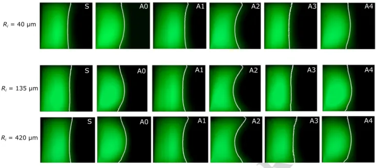
The location of the dyed stream is identified in Fig. 2. At the Y-junction, the two streams each occupy half of the channel width, separated by a straight centred interface in the plane of the channel cross-section. This interface is broadened by diffusion as the fluid travels downstream, and deformed in the region of the loops as the vortices of secondary flows transport fluid in the plane of the cross-section. Following the evolution of this interface by taking slices in the yz plane is thus a means of visualising the fluid transport that has occurred in the cross-sectional plane between consecutive slices. This evolution is shown in Fig. 6 for three channels with different inner radii of curvature, at the six locations identified in Fig. 2. The interface between the two streams of fluid is quite broad, due to molecular diffusion of the dye, but also due to the convolution of the image with a finite-sized point spread function, enhanced by the strong illumination conditions. Therefore, only the qualitative evolution of the interface can be obtained, by adjusting the light intensity at each z position with a diffusion-type profile. The inflection point of this profile provides an estimate of the location of the interface, which is marked by the bright lines in Fig. 6. This diffusion profile is wider towards the top and bottom, suggesting that Taylor dispersion is active in our system (Ismagilov et al. 2000). Coupled with the weaker light intensity close to the walls, this effect is responsible for a loss of resolution at the top and bottom wall, causing the slight bending of the interface observed in the straight channel (location S).

The top row in Fig. 6 shows the evolution of the interface in the channel we used for the μPIV measurements, at the largest De^∗ we investigated (0.86). This evolution is in good qualitative agreement with the numerically uncovered nature of the secondary flow as illustrated in Fig. 3a: between location S and A0, the fluid has travelled a quarter loop with the dyed stream at the inner edge of the bend. The convex shape of the interface at A0 indicates that the dye has been trans- ported towards the outer edge in the centreplane, and that un-dyed fluid has been carried towards the inner edge at the top and bottom walls. This is consistent with the transport expected from the numerically computed vortex structure.

From A0 to A1, transport along a quarter loop of reversed

394 395 396 397 398 399 400 401 402 403 404 405 406 407 408 409 410 411 412 413 414 415 416 417 418 419 420 421 422 423 424 425 426 427 428 429 430 431 432 433 434 435 436 437 438 439 440 441 442 443 444

445 446

447 448 449 450 451 452 453 454 455 456 457 458 459 460 461 462 463 464 465 466 467 468 469 470 471 472 473 474 475 476 477 478 479 480 481 482 483 484 485 486 487 488 489 490 491 492 493 494 495 496

(9)

UN CORRECTED PR

OOF

curvature leads to the recovery of a straight interface, which is bent to a concave shape after further transport in the same half loop to location A2. The channel then reverses curvature again, and a convex interface is observed after transport over half a loop (location A4). The images at A0, A2 and A4 are taken at the connection between consecutive half- loops, were the channel reverses curvature. An additional secondary flow is expected to be triggered from this sudden change in curvature even in a Newtonian fluid (Guglielmini et al. 2011). However, the displacement of the interface is not sensitive to the local velocity field, but rather to the integration of the streamlines over the distance travelled in the channel. Therefore, we expect that this is the reason we do not seem to observe the signature of this secondary flow in the cross-sectional profiles measured.

We will now use confocal visualisation to probe the influence of the radius of curvature of the channel R_i on the secondary flow, to gather further experimental proof of the flow scaling with De. As the relative magnitude of the secondary flow decreases for larger R_i , direct velocity measurements are difficult for those geometries. However, the integration over long distances makes the secondary flow visible in confocal experiments. The second and third rows in Fig. 6 show the evolution of the dyed and un-dyed streams interface in two channels of larger radii of curvature: R_i=135 μ m (middle row) and R_i=420 μ m (bottom row), but similar cross-section as the previous

channel. Q_insta depends non-linearly on R_i , therefore, for those two larger channels we do not work in terms of quan- tities scaled on the critical values, such as De^∗ . We keep the flow rate constant, so that the ratio of the Deborah numbers for both experiments is inversely proportional to that of the channel radii: De₁∕De₂=R_i,2∕R_i,1 . Confo- cal imaging of the cross-section shows clear evidence of the cross-sectional vortices, with marked deflections of the interface. The interface profiles obtained with the two larger channels have similar curvature, which provides semi-quantitative experimental evidence for the scaling of u_y with De: the displacement of the interface between, for instance, S and A0, is proportional to u_y×𝛥t , where 𝛥t is the time required for the base flow to travel from S to A0. 𝛥t∼R_i∕U∼R_i∕Q because the channels have the same cross-section. Therefore, the lateral displacement of the interface scales as u_y×R_i∕Q . As this displacement is similar for the two channels, and Q is identical, u_y scales as 1∕R_i , which is consistent with the linear scaling of u_y with De as measured numerically.

Finally, we also note that in all cases, the shape of the interface is almost unchanged after transport over an even number of consecutive half-loop (see A0 compared with A4). We thus confirm experimentally for Deborah numbers below one, memory effects are small in our system, as predicted numerically (Poole et al. 2013).

A4

S A0 A1 A2 A3

A4

S A0 A1 A2 A3 A4

Ri = 40 µm

Ri = 135 µm

Ri = 420 µm

Fig. 6 Top row: evolution of the cross-sectional view down the channel for the polymeric solution flown at De^∗=0.86 in the channel used for the μPIV experiments: the white line highlights the position of the interface, as obtained by adjusting the horizontal diffusion profile of the dye. Middle and bottom rows: effect of the radius of curvature of the channel. Q=14 μl/min, Ri=135 μ m (middle row) and

Ri=420 μ m (bottom row). Although the relative magnitude of the secondary flow is weaker than in the smaller channel, the larger Q and the integration over a longer distance make the vortical structure clear. The similarity of the interface evolution for both radii supports the scaling of the secondary flow with De

497 498 499 500 501 502 503 504 505 506 507 508 509 510 511 512 513 514 515 516 517 518 519 520 521 522 523

524 525 526 527 528 529 530 531 532 533 534 535 536 537 538 539 540 541 542 543 544 545 546 547 548 549

(10)

UN CORRECTED PR

OOF

1 3

Page 9 of 10 _####_

4 Conclusions and outlook

The use of two complementary techniques, μPIV in the centreplane of the microfluidic device and confocal microscopy to image the cross-section of the device, has allowed us to perform one of the first experimental char- acterizations of steady, viscoelastic secondary flows in curved microchannels. The vortical structure of this flow in the cross-sectional plane, first unveiled by numerical calculations, was confirmed. Qualitative agreement is found in the flow profiles for the secondary transverse velocity. Those results improve our comprehension of viscoelastic flows in complex channel geometries, by validat- ing the three-dimensional flow driven by the hoop stress in regions of constant curvature. A full understanding of the flow pattern in the serpentine channel, though, remains beyond the scope of our work: in the regions where the curvature is not constant (as is typically the case between consecutive half-loops), additional vortices may appear, which we do not discuss here. Their contribution to the flow dynamics in the serpentine microchannel may be important, though, via their interaction with the viscoelastic Dean flow we have characterised, and their position at a potentially critical location for the propagation of the elastic instability in the channel.

Acknowledgements AL and LD acknowledge funding from the ERC Consolidator Grant PaDyFlow (Grant Agreement no. 682367). RJP acknowledges funding for a “Fellowship” in Complex Fluids and Rhe- ology from the Engineering and Physical Sciences Research Council (EPSRC, UK) under grant number EP/M025187/1, and support from Chaire Total. SJH, AQS and LD gratefully acknowledge the support of the Okinawa Institute of Science and Technology Graduate University (OIST) with subsidy funding from the Cabinet Office, Government of Japan, and funding from the Japan Society for the Promotion of Science (Grant nos. 17K06173, 18H01135 and 18K03958). SL acknowledges funding from the Institut Universitaire de France. We would also like to acknowledge discussions on the nature of the secondary flow with Philipp Bohr and Christian Wagner. This work has received the support of Institut Pierre-Gilles de Gennes (Équipement d’Excellence,

“Investissements d’avenir”, program ANR-10-EQPX-34).

References

Afik E, Steinberg V (2017) On the role of initial velocities in pair dispersion in a microfluidic chaotic flow. Nature Commun 8(1):468

Afonso AM, Oliveira PJ, Pinho FT, Alves MA (2009) The log-conformation tensor approach in the finite-volume method framework.

J Non-Newton Fluid Mech 157(1–2):55–65

Afonso AM, Oliveira PJ, Pinho FT, Alves MA (2011) Dynamics of high-Deborah-number entry flows: a numerical study. J Fluid Mech 677:272–304

Alves MA, Oliveira PJ, Pinho FT (2003a) A convergent and universally bounded interpolation scheme for the treatment of advection. Int J Numer Meth Fluids 41:47–75

Alves MA, Oliveira PJ, Pinho FT (2003b) Benchmark solutions for the flow of Oldroyd-B and PTT fluids in planar contractions. J Non-Newton Fluid Mech 110:45–75

Amini H, Sollier E, Masaeli M, Xie Y, Ganapathysubramanian B, Stone HA, Di Carlo D (2013) Engineering fluid flow using sequenced microstructures. Nature Commun 4:1826

Amini H, Lee W, Di Carlo D (2014) Inertial microfluidic physics.

Lab Chip 14(15):2739–2761

Arratia PE, Thomas C, Diorio J, Gollub JP (2006) Elastic instabilities of polymer solutions in cross-channel flow. Phys Rev Lett 96(14):144502

Bird RB, Armstrong RC, Hassager O (1987) Dynamics of polymeric liquids, 2nd edn. Wiley, Hoboken

Bohr P, John T, Wagner C (2018) Experimental study of secondary vortex flows in viscoelastic fluids. arxiv pp 1–21

Burshtein N, Zografos K, Shen AQ, Poole RJ, Haward SJ (2017) Inertioelastic flow instability at a stagnation point. Phys Rev X 7(4):1–18

Casanellas L, Alves MA, Poole RJ, Lerouge S, Lindner A (2016) The stabilizing effect of shear thinning on the onset of purely elastic instabilities in serpentine microflows. Soft Matter 12(29):6167–6175

Dean W (1928) Lxxii, the stream-line motion of fluid in a curved pipe (second paper). Lond Edinb Dublin Philos Mag J Sci 5(30):673–695

Dean WR (1927) Xvi, note on the motion of fluid in a curved pipe.

Lond Edinb Dublin Philos Mag J Sci 4(20):208–223

Debbaut B, Avalosse T, Dooley J, Hughes K (1997) On the development of secondary motions in straight channels induced by the second normal stress difference: experiments and simulations.

J Non-Newton Fluid Mech 69(2–3):255–271

Del Giudice F, D’Avino G, Greco F, De Santo I, Netti PA, Maffettone PL (2015) Rheometry-on-a-chip: measuring the relaxation time of a viscoelastic liquid through particle migration in microchannel flows. Lab Chip 15:783–792

Di Carlo D (2009) Inertial microfluidics. Lab Chip 9(21):3038–3046 Di Carlo D, Irimia D, Tompkins RG, Toner M (2007) Continuous

inertial focusing, ordering, and separation of particles in microchannels. Proc Natl Acad Sci 104(48):18892–18897

Fan Y, Tanner RI, Phan-Thien N (2001) Fully developed viscous and viscoelastic flows in curved pipes. J Fluid Mech 440:327–357 Fani A, Camarri S, Salvetti MV (2013) Investigation of the steady

engulfment regime in a three-dimensional t-mixer. Phys Fluids 25(6):064102

Furukawa R, Arauz-Lara JL, Ware BR (1991) Self-diffusion and probe diffusion in dilute and semidilute aqueous solutions of dextran. Macromolecules 24(2):599–605

Gervang B, Larsen PS (1991) Secondary flows in straight ducts of rectangular cross section. J Non-Newton Fluid Mech 39(3):217–237

Groisman A, Steinberg V (2000) Elastic turbulence in a polymer solution flow. Nature 405:53–55

Guglielmini L, Rusconi R, Lecuyer S, Stone H (2011) Three-dimensional features in low-reynolds-number confined corner flows. J Fluid Mech 668:33–57

Hardt S, Drese KS, Hessel V, Schönfeld F (2005) Passive micromixers for applications in the microreactor and 𝜇TAS fields. Microfluid Nanofluid 1(2):108–118

Holyst R, Bielejewska A, Szymański J, Wilk A, Patkowski A, Gapiński J, Zywociński A, Kalwarczyk T, Kalwarczyk E, Tabaka M (2009) Scaling form of viscosity at all length-scales in poly (ethylene glycol) solutions studied by fluorescence correlation spectros- copy and capillary electrophoresis. Phys Chem Chem Phys 11(40):9025–9032

Ismagilov RF, Stroock AD, Kenis PJ, Whitesides G, Stone HA (2000) Experimental and theoretical scaling laws for transverse diffusive

AQ4 550

551 552 553 554 555 556 557 558 559 560 561 562 563 564 565 566 567 568 569 570 571 572 573

574 575 576 577 578 579 580 581 582 583 584 585 586 587 588

589

590 591 592 593 594 595 596 597 598 599 600 601

602 603 604 605 606 607 608 609 610 611 612 613 614 615 616 617 618 619 620 621 622 623 624 625 626 627 628 629 630 631 632 633 634 635 636 637 638 639 640 641 642 643 644 645 646 647 648 649 650 651 652 653 654 655 656 657 658 659 660 661 662 663 664 665 666 667

(11)

UN CORRECTED PR

OOF

broadening in two-phase laminar flows in microchannels. Appl Phys Lett 76(17):2376–2378

Kockmann N, Föll C, Woias P (2003) Flow regimes and mass transfer characteristics in static micromixers. Microfluid BioMEMS Med Microsyst Int Soc Opt Photon 4982:319–330

Lauga E, Stroock AD, Stone HA (2004) Three-dimensional flows in slowly varying planar geometries. Phys Fluids 16(8):3051–3062 0306572

Lee CY, Chang CL, Wang YN, Fu LM (2011) Microfluidic mixing: a review. Int J Mol Sci 12(5):3263–3287

Li XB, Oishi M, Oshima M, Li FC, Li SJ (2016) Measuring elasticity- induced unstable flow structures in a curved microchannel using confocal micro particle image velocimetry. Exp Therm Fluid Sci 75:118–128

Meinhart CD, Wereley ST, Gray MHB (2000) Volume illumination for two-dimensional particle image velocimetry. Meas Sci Technol 11:809–814

Mitchell P (2001) Microfluidics-downsizing large-scale biology. Nature Biotechnol 19(8):717

Mustafa MB, Tipton DL, Barkley MD, Russo PS, Blum FD (1993) Dye diffusion in isotropic and liquid-crystalline aqueous (hydroxypropyl) cellulose. Macromolecules 26(2):370–378

Oldroyd J (1950) On the formulation of rheological equations of state.

Proc R Soc London A 200:523–541

Ottino JM (1989) The kinematics of mixing: stretching, chaos, and transport, vol 3. Cambridge University Press, Cambridge Poole RJ, Lindner A, Alves MA (2013) Viscoelastic secondary flows in

serpentine channels. J Non-Newton Fluid Mech 201:10–16 Robertson AM, Muller SJ (1996) Flow of Oldroyd-B fluids in curved

pipes of circular and annular cross-section. Int J Non-linear Mech 31(1):1–20

Salipante P, Hudson SD, Schmidt JW, Wright JD (2017) Microparticle tracking velocimetry as a tool for microfluidic flow measurements.

Exp Fluids 58(7):1–10

Souliès A, Aubril J, Castelain C, Burghelea T (2017) Characterisation of elastic turbulence in a serpentine micro-channel. Phys Fluids 29:083102

Stroock AD, Dertinger SKW, Ajdari A, Mezić I, Stone HA, Whi- tesides GM (2002) Chaotic mixer for microchannels. Science 295(5555):647–651

Sznitman J, Guglielmini L, Clifton D, Scobee D, Stone HA, Smits AJ (2012) Experimental characterization of three-dimensional corner flows at low Reynolds numbers. J Fluid Mech 707:37–52 Tabeling P (2005) Introduction to microfluidics. Oxford University

Press on Demand, Oxford

Wereley ST, Meinhart CD (2005) Micron-resolution particle image velocimetry. In: Breuer KS (ed) Microscale diagnostic techniques.

Springer, Heidelberg, pp 51–112

Xue SC, Phan-Thien N, Tanner RI (1995) Numerical study of secondary flows of viscoelastic fluid in straight pipes by an implicit finite volume method. J Non-Newton Fluid Mech 59(2–3):191–213 Zilz J, Poole RJ, Alves M, Bartolo D, Lindner BLA (2012) Geometric

scaling of a purely elastic flow instability in serpentine channels.

J Fluid Mech 712:203218

Publisher’s Note Springer Nature remains neutral with regard to jurisdictional claims in published maps and institutional affiliations 668

669 670 671 672 673 674 675 676 677 678 679 680 681 682 683 684 685 686 687 688 689 690 691 692 693 694 695 696 697 698

699 700 701 702 703 704 705 706 707 708 709 710 711 712 713 714 715 716 717 718 719 720 721

722 723

724