橋梁マネジメントにおける有限要素曲面回帰(モデリングと最適化の理論)

橋梁マネジメントにおける有限要素曲面回帰

Finite

Element

Surface

Fitting

Algorithms for

Bridge Management

陳小君 木村拓馬

Xiaojun Chen Ibkuma Kimura

弘前大学理工学部数理科学科

Department of Mathematical Sciences, Hirosaki University

1.

Introduction

In the study of bridge deterioration, it is important not only to consider structural

evaluations and traffic load but also environmental factors such

as

climate and frequency

of earthquakes. However, such studies requireextensivedata sets andmethods forhandling

them. In the United States, the National Bridge InventoryDatabase (NBI) contains data

on over

600,000 bridges for

a

span of

33

years. In the past few years, there has been

a

growinginterest inthe study ofdataminingmethodsfor efficiently using NBI database with

Geographic Information System (GIS) database toanalyzeand predict bridge deterioration

[1]. The safety ofbridges in Japan is also crucial for the national trafic network. Japan

has

more

than 1,000 islands which form

a

long chain-like island

arc

surrounded by the Pacific

Ocean

and the Sea ofJapan. InJapan, there existextensive database thatcontains detailed historical data

on

over

672,000 bridges. Moreover, environmental factors have

great impacttobridges. To utilize theextensivebridge databasecombined with very large

geographic data sets,

we

have to developefficient surface fitting methods.

Geographicdatasets

are

oftenmade atirregularly spaced pointsand havemeasurement

errors.

Toanalyzethe irregularly spaced noisy data,manyinterpolationmethodsand

least-squares smooth fitting methods have been developed. Our aim is to efficiently

use

very

large datasets. In this paper,

we

studyfinite element discretization with

a

preconditioned

Newton method to find

an

approximation of a smooth function which minimizes

a

sum

of data residuals and the second derivative in $H^{2}(\Omega)$ under some constraints on data.

The discretizationresults

a

largescale constrained quadratic program whichinvolves large

sparse matrices.

We

show the quadratic

program

has

a

unique

solution

and propose

a

preconditioned Newton method to findthe solution.

Aomori Prefecture is located

on

the northernmost tip of Hunshu Island, Japan. It

is bordered by the Sea of Japan(west), the Pacific Ocean(east), and the Tsugaru

Chan-nel(north). There

are 1646

bridges in Aomori Region, in which 734 bridges

are

managed

by Aomori Prefecture. See Figure 1. Environmental factors have significant impact to

these bridges. We

use

the proposed method to form surfaces

over

Aomori Region by geo

value, earthquake magnitude, etc. Using these expanded data sets, wecan investigate the relation between environmental factors and bridge deterioration by data mining methods [1].

2.

Finite element

surface

fltting

Let St $\subset \mathbb{R}^{2}$be

a

convex

bounded domain. Thegivendata

are

measurementpoints

$\mathrm{x}_{i}=$

$(x_{1,1}, x_{1,2})\in\Omega$ and corresponding real values $y_{i},$ $i=1,2,$$\ldots n$

.

In

a

cartesian coordinate

system, the $x:,1$ and $x_{i,2}$ coordinates reflect the longitude and latitude, while the real

value$y_{i}$ may reflect rainfall value

or

earthquake magnitude at point $\mathrm{x}_{i}$

.

We

assume

that

$\mathrm{x}_{\dot{*}},$$i=1,2,$

$\ldots,$$n$arenot collinear (i.e., they do not all lieon

a

linein

$\Omega$). Let $S=\{\sim,i=$

$1,2,$$\ldots,$$n\}$ be the set of all measurement points, and $S_{0}\subset S$ be

a

subset of$S$

.

We considerthe following minimization problem,

$\min$ $\frac{1}{n}\sum_{1=1}^{n}(f(\sim)-y_{i})^{2}+\alpha|f|_{H^{2}(\Omega)}^{2}$

(1)

$\mathrm{s}.\mathrm{t}$

.

_{$f(*)\geq\tilde{y}:$}, _{$\sim\in S_{0}$}

over

all functions $f$ in the Sobolev space $H^{2}(\Omega)$

.

Here $\tilde{y}$

:

are

input data related to

$y_{i}$ and

a is

a

fixed positive parameter. The minimizer of (1) not only depends

on

the given data

$\ ,y_{*}$ and $\tilde{y}_{1}$, but also

on

the parametera. An appropriate choice of$\alpha$depends

on

the size

of the data.

In the

case

where $S_{0}$ is empty, the minimizer of (1) is called

a

thin plate spline. It

has been shown byDuchon[6] that there exists

a

unique thin platespline in $H^{2}(\Omega)$

,

when

$\Omega=\mathbb{R}^{2}$

.

Moreover,

numerical methods for finding approximate thin plate splines using

simplefinite element spaces in$H^{2}(\Omega)$have beenstudied. However, thereare

some

technical

problems to

use

standard thin plate splines for applicationsthat have large data sets. To

dealwith largedata sets, Christen, Roberts,Hegland andAltas $[5, 7]$proposed

a

methodto

find

a

finite

element thin plate splinein$H^{1}(\Omega)$

.

Intheirmethod,onlyfirst order derivatives

occur,

so

that simplefinite element spaces in$H^{1}(\Omega)$

can

be used to discretize theproblem.

Inmany applications,

some

constraints

on

data

are

required. Forinstance, at

measure-ment points, snowfall values

can

not be negativeorless thancertain values. Furthermore,

in

some

case,

we

do not know the exact values at

some

measurement points. Only upper

or

lowerbounds of these values

are

available. Hence it isnecessaryto study the

case

where

$S_{0}$ is nonempty. In this paper, we generalize the finite element approximation technique

for the thin plate spline in [7] and defineadiscretization problem of(1). Weintroduce

new

vector variable$\mathrm{u}=(u_{1},u_{2})$ which represents the gradient of the function $f$in (1), that is,

Moreover, we generalize the normalization condition

$\sum_{\dot{*}=1}^{n}(f(\sim)-y_{i})=0$

for thecase $S_{0}=\emptyset$ to

$\sum_{\mathrm{X}:\not\in s_{0}}(f(\mathrm{x}_{i})-y_{*}.)=0,$

$f(x_{i})-\tilde{y}_{i}\geq 0,$ $\mathrm{x}_{i}\in S_{0}$

.

(3)

Suppose that $S_{0}=\{\mathrm{x}_{n-t+1}, \ldots,\mathrm{x}_{n}\}$

,

where $r\geq 0$ ( $r=0$

means

$So=\emptyset$).

Now

we

consider

an

associated function $\mathrm{u}\in H^{2}(\Omega)$ satisfies

$f(\mathrm{x})=u(\mathrm{x})+\mu$ and $\sum_{:=1}^{n-f}u(\ )=0$

where $\mu$ is

a

constant. From (3)

we

have $\mu=\frac{1}{\hslash-f}\sum_{i=1}^{n-\mathrm{r}}y_{i}$

.

This leads to the following

minimization problem:

$\min$ $\frac{1}{n}.\sum_{*=1}^{n}(u(\mathrm{x}_{1})+\mu-y:)^{2}+\alpha(|u_{1}|_{H^{1}(\Omega)}^{2}+|u_{2}|_{H^{1}(\Omega)}^{2})$

$\mathrm{s}.\mathrm{t}$

.

$($Vu,$\nabla v)_{L^{2}(\Omega)^{2}}=(\mathrm{u},\nabla v)_{L^{2}(\Omega)^{2}}$, $\forall v\in H^{1}(\Omega)$

$\sum_{i=1}^{n-\mathrm{r}}u(\sim)=0$ (4)

$u(\mathrm{x}\iota)+\mu\geq\tilde{y}_{\dot{*}}$

,

$i=1,2,$ $\ldots,r$

over

allfunctions$u,$$u_{1},$$u_{2}\in H^{1}(\Omega)$

.

Inthis problem, $u_{1}$ and$u_{2}$

are

approximations of$\frac{\partial u}{\partial x_{1}}$

and $\frac{\partial u}{\partial x_{2}’}$ respectively. The purpose in introducing auxiliary functions

$\mathrm{u}_{1}$ and $u_{2}$ is for

the

use

of simple finite element spaces in $H^{1}(\Omega)$

.

In particular,

we use

simple continuous

piecewise polynomial spaces $\Omega^{h}\subset H^{1}(\Omega)$ associated with

a

finite element mesh

over

the

domain$\Omega$

.

Let $\mathrm{b}(x)=(b_{1}(x), \ldots,b_{m}(\mathrm{x}))^{T}$ denote

a

vector of basis functions for $\Omega^{h}$

.

Then func-tions $\mathrm{u},$$u_{1},$ $u_{2}$

are

given by

$\mathrm{u}(\mathrm{x})=\mathrm{b}(\mathrm{x})^{T}c$, $u_{1}(\mathrm{x})=\mathrm{b}(\mathrm{x})^{T}g_{1}$, $u_{2}(\mathrm{x})=\mathrm{b}(\mathrm{x})^{T}g_{2}$,

where the vectors $c,g_{1},g_{2}\in \mathbb{R}^{m}$ represent the linear combination coefficients in the basis

$\mathrm{b}$

.

Usingthe following matrix _{$N=(b:(x_{j}))\in \mathbb{R}^{n\mathrm{x}m}$},

we

can

define the values of

$u,$$u_{1},$$u_{2}$

at points$x_{l},i=1,2,$$\ldots,n$

,

by

$u(\mathrm{r})=(Nc):$, $u_{1}(n)=(Ng_{1})_{i}$, $u_{2}(\mathrm{r})=(Ng_{2}):$

.

Let matrices $A,$$B_{1},$$B_{2}\in \mathbb{R}^{m\mathrm{x}m}$be given by

Set $P=(0_{r\mathrm{x}(n-r)}, I_{r\mathrm{x}r})\in \mathbb{R}^{r\mathrm{x}n}$

.

Let $e_{n}\in R^{n}$ and $e_{f}\in R^{r}$ be the vectors whose $\mathrm{e}1\triangleright$

ments are all ones. For the corresponding data $y_{i}$, we set $\mathrm{y}=(y_{1}\cdots y_{n})^{T}\in \mathbb{R}^{n}$, $\tilde{\mathrm{y}}=$

$(\tilde{y}_{1}\cdots\tilde{y}_{\mathrm{r}})^{T}\in \mathbb{R}^{r}$

.

Now, we can write the finite element surface fitting problem

as

a

con-strained optimization problem in $\mathbb{R}^{3m}$,

$\min$ $\frac{1}{n}||Nc+\mu e_{n}-\mathrm{y}||_{2}^{2}+\alpha(g_{1}^{T}Ag_{1}+g_{2}^{T}Ag_{2})$

$\mathrm{s}.\mathrm{t}$

.

$Ac=B_{1}g_{1}+B_{2}g_{2}$ (5)

$(e_{n}^{T}-e_{f}^{T}P)Nc=0$

$PNc+\mu e_{r}\geq\tilde{\mathrm{y}}$

It is worth noting that the number of variables $(c,g_{1},g_{2})\in \mathbb{R}^{3m}$ depends

on

the

dis-cretization of a finite element mesh, but not

on

the size of data. Moreover, matrices

$A,$$B_{1},$$B_{2}\in \mathbb{R}^{m\mathrm{x}m}$and $N\in \mathbb{R}^{n\mathrm{x}m}$

are

sparse.

3. Preconditioned Newton

method

In this section,

we

show that problem (5) has

a

solution and present

a

preconditioned

Newton method for solving (5).

Let

$W=$

.

For any given$g_{1},g_{2}\in \mathbb{R}^{m},$ $c$ can be obtainedby the equality constraints inproblem (5) as

$c=W^{+}$

,

where $W^{+}$ is the generalized inverse of _$W[2]$ which satisfies $W^{+}W=I\in \mathbb{R}^{m\mathrm{x}m}$

.

Let

$W_{1}^{+}\in \mathbb{R}^{m\mathrm{x}m}$ be the submatrix of$W^{+}$ whose entries lie in the first _$m$ columns. Then

we

have $c=W_{1}^{+}(B_{1g_{1}}+B_{2g_{2}})$

.

Let us denote

$g=$

,

$G=NW_{1}^{+}(B_{1}, B_{2}),$

$H=$

.

Then problem (5) reducesto the following optimization problem

$\min$ $\frac{1}{n}||Gg+\mu e_{n}-\mathrm{y}||_{2}^{2}+\alpha g^{T}Hg$

(6)

$\mathrm{s}.\mathrm{t}$

.

$PGg+\mu e_{f}\geq\tilde{\mathrm{y}}$

.

The objectivefunction in (6)

can

be rewritten

as

Let $Z=W_{1}^{+}N^{T}NW_{1}^{+}$

.

The matrix

$Q:=G^{T}G+n\alpha H=$

is symmetric positive definite. Therefore, the objectivefunction in (6) is strongly convex,

and

problem (6) has

a

unique solution.

By

convex

optimization theory, problem (6) is equivalent to the following system of

nonsmoothequations

$F(z)==0$

(7)

where$z=(g, \lambda)$ and A $\in R^{f}$ is the Lagrangemultiplier.

To solve (7),

we use

the generalized Newton method,

$z^{k+1}=z^{k}-V_{k}^{-1}F(z^{k})$ (8)

where $V_{k}$ is

an

element in the generalized Jacobian of $F$ at $z^{k}[4]$

.

Moreover, at each

iteration of (8),

we use a

preconditioned Uzawa method [3] to solve the system of linear

equations

$V_{k}d=-F(z^{k})$

.

(9)

We

can

show that this methodsuperlinearly

converges

to

a

solution $z^{*}$ of(7), that is, $\lim_{\mathrm{k}arrow\infty}\frac{||z^{k+1}-z^{*}||}{||z^{k}-z^{*}||}=0$

.

(10)

Moreover, it

can

be shown that there is

a

constant $\kappa$ suchthat for any $z\in R^{2m+\gamma}$

,

$||z-z^{*}||\leq\kappa||F(z)||$

.

(11)

This

error

bound

can

be used to examine how measurement errors in the data affect

predicated values.

4.

Numerical experiment

In the United States, data mining methods have beenused to efficiently

access

bridge

inventory database and geographic information for the study of bridge deterioration [1].

The

KITACON

company inspects bridges in

Aomori

Region regularly and has structural evaluations and

traffic

records for all bridges managed by

Aomori

Prefecture. In order to

use efficient data mining methods for bridge management,

we

need environmental data,

used the finite element surface fitting method proposed in previous sections and climate

data from Japan Meteorological Agency to predicate some environmental data

on

every

bridge in Aomori Region.

Aomori Region is surrounded by water

on

all three sides, the Pacific Ocean to the

east, the Tsugaru Channel to the north and the seaof Japan to the west. Climate factors

have great impact to bridges in Aomori Region. We report

some

numerical results

on

temperature, snowdepth, rainfall in Figures 2-4.

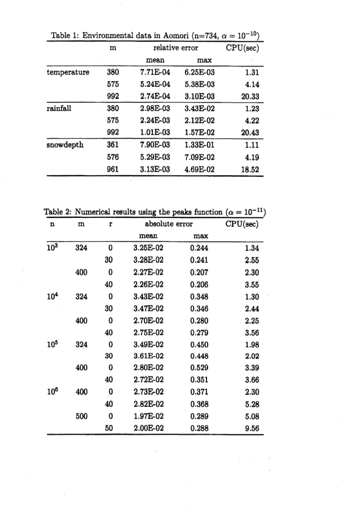
To verify the accuracy of the predicated environmental data

on

every bridge,

we use

these predicated data and the finite element surfacefittingmethodtodefine testing values

at the measurement points of Japan Meteorological Agency. Table 1 shows the relative

error

of the testing values to the true values at the measurement points.

Finally,

we use

the”peaks”

function

from Matlab to show that

our

finite elementsurface fitting method

can

handle very large data sets. The peaks function is formed

as a

linear

combination of several scaled and translated Gaussian distributions. Table 2 reports the

error

$= \frac{1}{n}\sum_{1=1}^{n}.|f(\mathrm{r})-y:|$for

a

data set of$n$pointswith

a

finite element grid of$m$ by $m$

.

Preliminary numericalresults indicate thatthe finiteelementsurface fitting method is

promising for handling very large data sets. The generalized Newton method is efficient

for solving (7). Computation time for solving (7)

are

shown in thble 1 and Table 2.

Computationswere performed by usingMatlab 7.0 on aIBM PC with IGB memory and

Pentium$4(3\mathrm{G}\mathrm{H}\mathrm{z})$

.

References

[1] S. B. Chase and E.P.Small, An in-depth analysis ofthe national bridge inventory database

utilizing data mining, GIS and advanced statistical methods, Transportation Research

Circu-lar 498(C6), Presentations of the 8th International Bridge Management Conference, Denver,

Colorado, 1999, 1-17.

[2] X. Chen, M.Z. Nashed and L. Qi, Convergence of Newton’s method for singularsmooth and

nonsmoothequations using outer inverses, SIAMJ. Optim., 7(1997) 445-462.

[3] X. Chen, Globalandsuperlinearconvergence ofinexactUzawa methods for saddlepoint

_Prok

lems with nondifrerentiablemappings,SIAM J. Numer. Anal. 35(1998) 1130-1148.

[4] F. H. Clarke, Optimization andNonsmooth Analysis, Wiley, NewYork, 1983.

[5] P. Christen,M.Hegland,S.RobertsandI.Altas, A scalableparallelFEM surfacefittingalgorithm

for data mining, Technical Report TR-CS-OI-OI, TheAustralian National University2001.

[6] J.Duchon,Splinesminimizingrotation-invariant semi-normsinSobolev$\mathrm{s}\mathrm{p}\mathrm{a}\varpi$, inConstructive

TheoryofFunctions ofSeveralVariables,Lecture Notes in Math. 571, 1977,85-100.

[7] S. Roberts, M.Helgland andI.Altas, Approximation ofathinplate splinesmootherusing

$\frac{\mathrm{T}\mathrm{a}\mathrm{b}\mathrm{l}\mathrm{e}1:\mathrm{E}\mathrm{n}\mathrm{v}\mathrm{i}\mathrm{r}\mathrm{o}\mathrm{n}\mathrm{m}\mathrm{e}\mathrm{n}\mathrm{t}\mathrm{a}\mathrm{l}\mathrm{d}\mathrm{a}\mathrm{t}\mathrm{a}\mathrm{i}\mathrm{n}\mathrm{A}\mathrm{o}\mathrm{m}\mathrm{o}\mathrm{r}\mathrm{i}(\mathrm{n}=734,\alpha=10^{-10})}{\mathrm{m}\mathrm{r}\mathrm{e}\mathrm{l}\mathrm{a}\mathrm{t}\mathrm{i}\mathrm{v}\mathrm{e}\mathrm{e}\mathrm{r}\mathrm{r}\mathrm{o}\mathrm{r}\mathrm{C}\mathrm{P}\mathrm{U}(\sec)}$

mean

$\max$

temperature

380

7.71E-04

6.

$25\mathrm{B}03$

1.31

575 5.24E-04 5.38E-03 4.14

992

2.74E-04 3.10E-03 20.33

rainfall

380

2.98E-03 3.43E-02 1.23

575

2.24E-03 2.12E-02 4.22

992

1.01E-03 1.57E-02

20.43

snowdepth $36l$ 7.90E-03 1.33E-0l 1.11

576

5.29E-03 7.09E-02

4.19

961

3.13E-03

4.

$69\mathrm{B}02$

18.52

Table 2: Numericalresults using the peaks function $(\alpha=10^{-11})$

$\mathrm{n}$ $\mathrm{m}$ $\mathrm{r}$ absolute

error

CPU(sec)

mean $\max$ $10^{3}$ 324 $0$ 3.25E-02

0.244

1.34

30

3.

$28\mathrm{B}02$

0.241

2.66

400

$0$ 2.27E-02

0.207

2.30

40

2.26E-02

0.206

3.55

$10^{4}$ 324 $0$ 3.43E-02

0.348

1.30

30

3.47E-02

0.346

2.44

400

$0$ 2.70E-02

0.280

2.25 40 2.$75\mathrm{B}02$

0.279

3.56

$10^{5}$ 324 $0$ 3.49E-02 0.450 1.98 30 3.61E-02 0.448 2.02 400 $0$ 2.80E-02

0.529

3.39 40 2.72E-02

0.351

3.66

$10^{6}$

400

$0$

2.

$73\mathrm{B}02$

0.371

2.30

40

2.82E-02

0.368

5.28

500

$0$ 1.97E-02 0.289 5.08

50

$2.00\mathrm{E}\cdot 02$

0.288

9.56

Figure 1: Distribution ofbridges in

Aomori

Figure 3: Values ofhighest snowdepth in

2005

(cm)