I. Introduction
A large body of literature has been accumulated on the measurement of marginal will- ingness to pay (MWTP) for non-market goods, such as environmental quality and neighbor- hood amenities, coupled with its policy implications. Many previous studies use a hedonic approach to measure the MWTP for non-market goods, under the assumption that the value of these non-market goods is capitalized into local housing prices.
Given that residential location choice often coincides with school choice, evaluating par- ent’s willingness to pay for school quality through housing valuations has been one of the most extensively investigated topics in the literature. An obvious empirical challenge is that there are often a number of housing and neighborhood unobservables that correlates both with housing values and with school quality. As a result, a number of alternative methods have been proposed to pin down the causal relationship between house prices and school quality. Comparing estimates based on different methodology allows us to understand po- tential biases and their underlying mechanisms in the hedonic applications. In addition, comparing results from different countries and/or institutional backgrounds can provide im- portant insights in terms of the generalizability of empirical findings (i.e., external validity).
Several comprehensive literature surveys have already been published in the last decade (Black and Machin, 2011; Machin, 2011; Nguyen-Hoang and Yinger, 2011). The purpose of this paper is therefore to review more recent studies and to discuss improvements and re-
School Quality and Residential Property Values: A Review of Recent De- velopments and Applications
NAOI Michio
Associate Professor, Faculty of Economics, Keio University
Abstract
The measurement of consumers’ marginal willingness to pay for public education pro- vides a basis for evaluating and improving existing education policies. This study reviews recent empirical studies that examined the relationship between school quality and housing prices based on a hedonic approach. We classify the existing empirical works according to their identification strategies, discuss the magnitudes of the estimated marginal willingness to pay for public education, and highlight several key aspects that need to be investigated in future research.
Keywords: School Quality, Property Value, Hedonic Approach
JEL Classification: C21; I21, H75; R23
finements of methodology over time.
The structure of this paper is as follows. The next section introduces the basic frame- work of the hedonic approach and presents the major empirical issues. Section III presents an empirical framework for several important existing studies, focusing particularly on bias- es resulting from inadequate control of the neighborhood unobservables. Section IV over- views recent research trends from three perspectives: identification strategies on empirical analysis, magnitude of MWTP estimates, and several key topics in the literature. Section V discusses the advantages and disadvantages of using Japanese data, drawing on several previous studies. Section VI concludes.
II. Hedonic Approach II-1. Basic Framework
Evaluating the value of non-market, neighborhood amenity has been an important topic in urban and environmental economics. Under the assumption that the value of neighbor- hood amenity is capitalized into local house prices, many previous studies have applied he- donic methods in order to evaluate the MWTP for neighborhood amenity (Rosen, 1974).
1In our case, house prices can be higher in the neighborhood of a good public school, reflecting consumers’ willingness to pay for good schools.
In the framework of the hedonic approach, individual houses represent not only a bundle of structural characteristics, such as size and age, but also a set of location-specific charac - teristics. These latter characteristics include, among others, accessibility, neighborhood housing and demographic composition, and local public goods such as schools. Let s be the quality of local public school and all other structural and location-specific characteristics be z = ( z
1, z
2,…, z
A). Thus, individual houses are characterized by the bundle of characteristics (s, z).
Consumers are assumed to derive utility from a bundle of housing characteristics (s, z) and numeraire goods consumption ( x ). They have utility function U ( x , s , z; ξ ) where ξ is a parameter representing the consumer’s heterogeneity. The consumer’s budget constraint is given by y = x + P(s, z) where y is income and P(s, z) is an equilibrium hedonic price func- tion, i.e., housing value given its characteristics. The first-order condition describing the consumer’s hedonic demand yields
(1) The left-hand side of the equation is the implicit price of school quality, i.e., the marginal
U
s( y – P (s, z), s, z ; ξ ) U
x( y – P (s, z), s, z ;ξ )
P
s(s, z) = .
1 In this paper, we focus mostly on the identification of “marginal” willingness to pay for school quality. Evaluating the wel- fare impact of “non-marginal” changes in school quality often requires more structural approach such as Rosen’s classic two- stage procedure. Empirical issues and the recent development on identifying the non-marginal impact of location-specific char- acteristics can be found, for example, in Ekeland et al. (2004), Bajari and Benkard (2005), and Heckman et al. (2010).
impact of school quality on house prices, which can in principle be estimated from the ob- served data. The right-hand side is the consumer’s MWTP for school quality. Equation (1) therefore provides theoretical rationale for identifying the consumer’s evaluation of school quality through housing valuation.
II-2. Empirical Issues
Suppose we can observe price p, school quality s and structural and location-specific characteristics z for houses i∈ {1, 2, …, N}. A standard hedonic price function is given as
log p
i= βs
i+ z
i′γ + ε
i(2)
where ε denotes an error term. As discussed in the previous section, the estimated coefficient β can be interpreted as MWTP for school quality. In the following, we will discuss major empirical issues in estimating hedonic price function given in equation (2). These include (1) measurement of the school quality s , and (2) omitted-variable bias due to unobserved neigh- borhood characteristics.
2Ⅱ-2-1. Measuring School Quality
In equation (2), s
irepresents the quality of educational services available for household i . In practice, however, an appropriate measure of school “quality” is not necessarily obvious.
Since education is a multifaceted good, there are a number of potential aspects that consti- tute the quality of public schools.
To address this issue, several recent studies look at the household’s school choice and examine how parents evaluate various school characteristics such as facilities, convenience or peer composition. For example, Burgass et al. (2015), using survey data on school choice in the UK, examine the school characteristics that influence the choice between public ele- mentary schools. Their empirical results suggest that parents have strong preference for schools’ academic performance (i.e., average scores on a standardized academic exam) and that more advantaged parents tend to value more on academic performance.
3More recently, Abdulkadiroglu et al. (2020) use school choice data in New York City and examine whether observed school choice is influenced by academic performance of the existing students (i.e., average test score) or by its value added (i.e., test score improvement). Their empirical re- sults show that, conditional on the average academic performance, schools’ value added does not have any additional influence on school choice. These empirical results imply that parents and families tend to value peer quality rather than school effectiveness.
Schools’ academic performance, either in its average or the value added, is a measure of school quality in terms of educational outcomes. Parents may also care about educational inputs such as schools’ facilities or teacher quality as a means of improving educational out-
2 In addition to the issues addressed here, the estimation of the hedonic price function involves a variety of empirical issues, including the choice of functional forms, spatial segmentation of housing submarkets, and various sample selection issues. For a broader discussion of the estimation of hedonic price functions, see Sheppard (1999) for example.
3 Their results suggest that parents also value schools’ accessibility and socio-demographic composition.
comes. There is also an extensive literature on the education production function that inves- tigates the determinants of educational outcomes. Previous studies examined the role of school resources, including student/teacher ratio, teachers’ education and years of experi- ence, educational expenditures per student, school facilities (Hanushek, 2006; Todd and Wolpin, 2003). Estimating the education production function per se has a number of data and empirical issues and the causal impacts of various school resources on student’s out- comes are still widely discussed in the literature. Despite the lack of empirical consensus on its impact on educational outcomes, school resources can still be one of the potential mea- sures of school quality.
Previous studies on school choice and education production function suggest that school quality in equation (2) can be measured by schools’ academic achievement (such as stan- dardized test scores) and/or by their educational resources (such as teacher quality). So far, however, much of the previous research in the hedonic literature has primarily used average test scores as a measure of school quality. This is perhaps due to the lack of readily available data for student’s academic value added or for detailed measures of school resources. Em- pirical results using value-added measures or school resources will be discussed later in Section IV.
Another empirical issue on the measurement of school quality relates to the spatial cor- respondence between residential location and available schools. Without open enrollment or school choice programs, residential location choice often coincides with the choice of a spe- cific school to be enrolled in, through attendance zoning or school boundary maps. In this case, spatial mapping between housing and schools will not be a problem. In some countries or regions, however, attendance zones are not always strictly enforced or such geographic attendance rules are nonexistent. In such a case, one has to care about parental school choice problems on top of residential location choice, which substantially complicates the standard hedonic analysis.
While institutional factors such as open enrollment or school choice programs can create difficulties in measuring school quality, they can also be an advantage in the empirical anal- ysis since the introduction of these programs provides exogenous variation in school quality at each location. Additional discussion of these issues will be provided in Section IV.
Ⅱ-2-2. Endogeneity Issues
In recent empirical studies using observational data, quasi-experimental designs for the identification of causal relationships have become more important than before. This trend is also true with respect to empirical analysis based on hedonic approaches, and much of the recent research has developed in a way that incorporates a wide variety of quasi-experimen- tal designs for causal inference (Parmeter and Pope, 2013; Ushijima, 2016).
In this context, a key concern in estimating equation (2) is the endogeneity of school
quality and its possible correlation with the unobserved omitted neighborhood characteris-
tics. In the presence of endogeneity, i.e., E[ε|s, z] ≠ 0, estimating equation (2) by the stan-
dard technique such as OLS will yield biased estimates and spurious findings. This will hap-
pen in a number of settings. First, higher housing prices can improve school quality (i.e., reverse causation). This can be particularly problematic in the public school system in the U.S., where school budgets are partly financed by local property taxes. The most recent fig- ures suggest that approximately 33.6% of U.S. education spending on public elementary and secondary schools is funded by school district’s property tax revenues.
4In this case, if higher house prices lead to higher property tax revenues, a high willing- ness to pay for school quality could lead to an increase in school spending. Since the U.S.
school system leaves much of school operation, such as teacher and staff personnel and school facility maintenance, to the discretion of school districts, increases in education bud- gets can directly result in improvements in school resources, and hence quality. Therefore, a reverse causation between house prices and school quality will create difficulties in the anal- ysis based on equation (2). Unfortunately, however, much of the previous studies are unable to deal with this reverse causation issue and assume that marginal home buyers do not sub- stantially change neighborhood characteristics and school quality (Black and Machin, 2011).
5Second, school quality can be strongly correlated with neighborhood characteristics due to residential sorting. If there are some unobserved characteristics correlated with school quality, a simple regression analysis based on equation (2) will provide a biased estimate of β. This omitted variables problem is widely recognized in the literature and several methods have been proposed. This point will be discussed in more detail in the next section.
III. Boundary Discontinuity Design
As discussed in the previous section, unobserved neighborhood characteristics can yield biased estimates of the impact of school quality on house prices. In the following, we look at several analytical methods proposed in existing research to address this issue.
Equation (2) assumes a situation in which variables that could affect house prices are fully observed by the econometrician. However, there are a myriad of structural and loca- tion-specific characteristics that can influence house prices, and the econometrician can al- most always observe an incomplete set of these characteristics. Suppose that a subset z ̴ = { z
1,
…, z
Ã} of the housing characteristics z can be observed by the econometrician (Ã < A). In this case, the regression equation that can actually be estimated is
log p
i= βs
i+ z ̴
i′ γ̴ + ε ̴
i(3)
where ε ̴ is an error term that includes housing characteristics that are unobservable to the econometrician (z
à + 1, …, z
A).
4 A breakdown by source of funds in FY 2015 shows that 55.2% of the total spending came from the federal or state govern- ment and 44.8% from smaller governmental units than the state, including school districts. A further breakdown of the latter shows that 81.3% came from property tax revenues, 14.9% from other public revenues, and 3.8% from donations and other revenues (Digest of Education Statistics 2018).
5 Some studies have addressed this issue using the instrumental variables method. For example, Downes and Zabel (2002) use the percentage of rental housing and school-age children in the local population as IV and estimate hedonic regression similar to equation (2). The validity of these IVs, however, remains controversial.
The bias due to the omitted neighborhood characteristics arises because the error term ε ̴ in equation (3) is correlated with school quality s (after conditioning z ̴ ). For example, neigh- borhood characteristics such as landscape is difficult to quantify and may be associated with school quality.
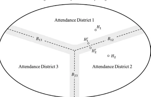
To circumvent the problem from omitted neighborhood characteristics, Black (1999) compares houses within a close proximity to each other but located on the opposite sides of school attendance zone boundaries. The basic idea of this method is as follows. Figure 1 shows three attendance zones within the same school district. Consider two houses, H
1and H
2, located in different attendance zones. Since two houses are located in different school districts, the price difference is at least partly due to differences in school quality. However, the two houses are also likely to have different neighborhood environments as they are lo- cated far apart. If these neighborhood environments are not fully observable, and if unob- servable elements of the neighborhood environment are correlated with school quality, then the observed price differences will reflect not only differences in school quality but also un- observable differences in the neighborhood environment (i.e., omitted variables bias).
In contrast, if we consider two houses, H
1′ and H
2′, within a very close proximity to each other, we can expect that two houses share almost the same neighborhood environment. At the same time, since two houses are still located in different school districts, the school qual - ity they face will be different. Therefore, any difference in house price can be attributed to differences in school quality.
Figure 1. Boundary Discontinuity Design
In a regression framework, Black (1999) estimates hedonic regressions to a sample of houses that are very close to the attendance zone boundaries. In Figure 1, this corresponds to limiting the sample to houses located in a gray area near the attendance zone boundaries.
If neighborhood characteristics other than school quality change smoothly at the district boundary, any discontinuous changes in house prices at the boundary are due to the discon- tinuous changes in school quality. Such an identification strategy is similar to the idea of re- gression discontinuity design, a quasi-experimental approach for policy evaluation, and is often referred to as boundary discontinuity (BD) design (Imbens and Lemieux, 2008; Lee and Lemieux, 2010).
The empirical results based on the BD approach show that a 5% increase (approximately one standard deviation) in average test scores would increase house prices by 1.3 to 1.6%.
In contrast, standard hedonic regression models using full samples show that house prices increase by about 3.5% for an equivalent change in average test scores. These results sug- gest that the presence of an unobservable neighborhood environment leads to a large upward bias in the estimates of β.
The method is clearly innovative and, as discussed below, much of the recent empirical work on the same topic has employed identification strategies based on the BD approach.
However, several problems have been recognized with this approach. One of the major problems concerns residential sorting across different school attendance zones. If families care about school quality and choose their residential location accordingly, the local socio- economic characteristics may change discontinuously at the attendance boundaries.
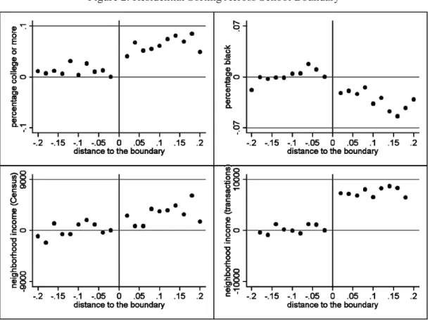
6Figure 2 summarizes the movement of neighborhood sociodemographic characteristics in the region of school attendance boundaries (Bayer et al., 2007). Bayer et al. (2007) focus on boundaries for which the gap in average test scores on each side of the boundary is great- er than the sample median (38.4 points). The figure shows average neighborhood sociode- mographics—share of college graduates and black, and average household income—calcu- lated at the census block level at a given distance to the school attendance boundary, where negative distances indicate the low test score side. On average, families in the high test score side of the boundary tend to have a higher education, earn a higher income, and are less likely to be black.
If households have preferences over their neighbors, residential sorting and discontinu- ous changes in neighborhood sociodemographic characteristics at the boundary can lead to biased BD estimates.
7Returning to the example in Figure 1, if households have preferences for the racial composition of the neighborhood, the price difference between two houses H
1′
6 Discontinuous changes in the neighborhood environment at attendance district boundaries can be caused by various reasons other than residential sorting. For example, when attendance district boundaries coincide with administrative boundaries, avail- able public services and/or tax rates may change discontinuously at the boundary. In addition, if adjacent school districts are physically separated from each other by rivers, large roads, or other factors, the neighborhood environment can change signifi- cantly at school district boundaries. Therefore, these cases should be carefully excluded in the analysis.
7 They extend the standard boundary discontinuity approach and develop a discrete-choice model of residential sorting, using boundary fixed effects for the identification of heterogeneous preferences for schools and neighborhoods. For more recent ap- plication of their approach, see Tra et al. (2013) for example.
and H
2′ near the attendance boundary would be affected not only by discontinuous changes in school quality but also by changes in racial composition of the neighborhood at the boundary.
Bayer et al. (2007) find that controlling for neighborhood sociodemographics (neighbor- hood racial composition and education) at the census block level yields substantially smaller BD estimates. Specifically, they show that the school quality effects on housing prices be- come approximately 50% smaller in BD models with neighborhood sociodemographic con- trols than in standard BD models with boundary fixed effects.
IV. Recent Empirical Evidence
In this section, we review major findings and methodological developments in recent empirical studies based on the hedonic approach. As mentioned earlier, given that several
Figure 2. Residential Sorting Across School Boundary
Source: Bayer et al. (2007, Figure 4).
Notes: The horizontal axis represents distance to the boundary, where negative values indicate the low test score side. The vertical axis represents average neighborhood sociodemographic characteristics for residents’ educa- tion (% college degree or more), racial background (% black), and household income. The lower left panel uses census-reported household income, and the lower right panel uses household income from transaction data.
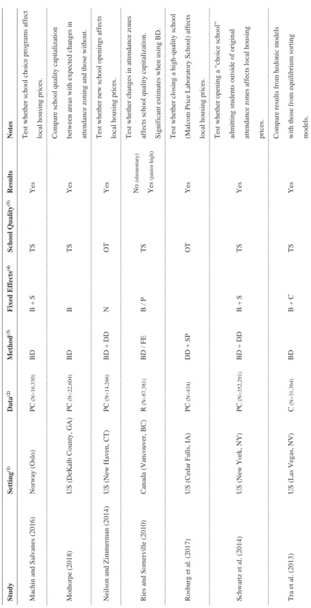
surveys already exist on this topic, our review here covers a list of empirical studies mostly published after 2010. We include studies published before 2009 if they are not covered by previous surveys, especially those on Japan. The studies covered are summarized in Table 1.
The following section provides an overview of the recent studies listed in Table 1 from three perspectives: identification strategies and empirical methods employed, the magnitudes of the MWTP estimates, and the specific research topics.
IV-1. Identification Strategies and Empirical Methods
As discussed in the previous section, the BD approach has become increasingly common in the literature. In fact, 17 of the 28 studies listed in Table 1 have employed BD design as the basic identification strategy. In contrast, Black and Machin (2011), which summarize studies prior to 2010, report that only 10 out of 54 papers in question employed a BD de- sign.
On top of that, there are two major methodological features observed in the recent stud- ies. First, even in empirical analyses that employ BD design as a basic identification strate- gy, an increasing number of studies are using some kind of time-series variation in school quality as an additional source of identification by using pooled transaction data from multi- ple points in time. For example, several papers employ a combination of BD and differ- ence-in-differences identification strategies by focusing on events such as new school open- ings or changes in the geography-based attendance rules (Neilson and Zimmerman, 2014;
Schwartz et al., 2014; Chung, 2015; Andreyeva and Patrick, 2017).
8These cases will be dis- cussed in more detail in Section Ⅳ-3-2.
Second, in response to the potential bias stemming from residential sorting, an increas- ing number of analyses control for neighborhood environments that can be correlated with school quality at the spatially disaggregated levels. Table 1 summarizes the spatial fixed ef - fects that are controlled for in the empirical analysis (see “Fixed Effects” column), showing that many studies include fixed effects at the census block levels or their equivalent.
A notable example from this perspective is by Ries and Sommerville (2010). They em- ploy an identification strategy that uses a time-series variation in school quality due to changes in school attendance zones, controlling for fixed effects at the housing unit level by using data on houses transacted multiple times during the sample period (i.e., repeat sales data). Their findings suggest that average test scores are positively associated with local house prices in the standard BD setting with boundary fixed effects, whereas BD estimates lose their statistical significance when controlling for housing unit-level fixed effects.
There are several recent papers that apply the “spatial differencing” approach that is built upon a standard BD model (Gibbons et al., 2013; Zheng et al., 2016). Suppose that the exact location of housing i is denoted by c
i(for example, by longitude and latitude). The
8 However, large-scale events such as school openings and changes in attendance rules can change the equilibrium of the he- donic model itself, and there are several discussions on whether β identified by the non-marginal changes in school quality caused by these events can be interpreted as a marginal willingness to pay (Kuminoff and Pope, 2014; Banzhaf, 2018).
StudySetting(1)Data(2)Method(3)FixedEffects(4)School Quality(5)ResultsNotes Agarwal et al. (2016)SingaporePC(N=135,788)DDNTSYesTest whether school relocation affectslocal housingprices. Andreyeva and Patrick (2017)US (Atlanta, GA)PC(N=28,654) R (N=22,860)BD+DDB + COTYesTest whether opening charter schools affects local housingprices. Beracha and Hardin III (2018)US (Miami, FL)PC(N=116,386(rental), N=198,747(sales))BDBTSYesCompare the capitalization of school quality on housing rents and transaction prices. Carrillo et al. (2013)US (Fairfax County,VA)C(N=37,258 (2001-2002), N=15,579 (2006-2007))BDSTSYes
Test whether school information disclosure on the multiple listing services (MLS) affects local housingprices. Chung (2015)South Korea(Seoul)PC(N=10,259(rental), N=28,182 (sales))BD + DDB+ POTYes
Test whether abolishment of geographic attendance rules affects local housing prices. Admission to the Seoul National U. as the measure of school quality. Clapp et al. (2008)US (CT)PC(N=356,829)FES + NTS + SDYesCompare results from various quality measures. Conlin and Thompson (2017)US (OH)PC(N=2,225)OTIPYes
Estimate the impacts of school’sfacility investment financed by the statesubsidy programon student outcomes. Dhar and Ross (2012)US (CT)PC(N=68,288)BDB + BSTSYesFocus on school district boundaries rather than attendance boundaries.
Table 1. Summary of Recent Empirical Findings
StudySetting(1)Data(2)Method(3)FixedEffects(4)School Quality(5)ResultsNotes Feng and Lu (2013)China (Shanghai)PC(N=2,496)FENOTYesTest whether designation of “core high schools”affects local housingprices. Fiva and Kirkebøen (2011)Norway (Oslo)PC(N=79,322)FESTSYes(short-run) No(long-run)
Test whether school information disclosure affects local housingprices. Fleishman et al. (2017)IsraelPC(N=5,666)FESTSYesTest whether disclosure of average test scores affects local housingprices. Gibbons and Silva (2011)UKC(N=560)FESTS +OTYesUse subjective assessment of schools by existing students and parents as school quality measures. Gibbons et al. (2013)UKPC(N=1,656,056)BD+SP +OTBTSYes(average) Yes(value-added)
Compare results using average test scores and value-added measures. Hwang et al. (2019)US (Pitt County, NC)PC(N=5,135)OTCTS + IPYesTake account of preference heterogeneity by employing finite mixture models. Imberman and Lovenheim (2016)US (Los Angeles, CA)PC(N=63,122)BD+DDSTS + IPYes(average) No (value-added)Test whether school information disclosure affects local housingprices. Kuroda (2018)Japan (Matsue, Shimane)C(N=2,642)BDBTSYes
Test whether average test scores from the nationwide exam (Zenkoku Gakuryoku Chosa) affects local housing rents. La (2015)US (Boston, MA)PC(N=20,674)BDNTSYesExploit distance-based assignment to the local public schools.
Table 1 (continued). Summary of Recent Empirical Findings
Table 1 (continued). Summary of Recent Empirical Findings
StudySetting(1)Data(2)Method(3)FixedEffects(4)School Quality(5)ResultsNotes Machin and Salvanes (2016)Norway (Oslo)PC(N=16,330)BDB + STSYesTest whether school choice programsaffect local housing prices. Mothorpe (2018)US (DeKalb County,GA)PC(N=22,604)BDBTSYesCompare school quality capitalization between areas with expected changes in attendance zoning and those without. Neilson and Zimmerman (2014)US (New Haven, CT)PC(N=14,266)BD+DDNOTYesTest whether new school openings affects local housingprices. Ries and Somerville (2010)Canada (Vancouver, BC)R(N=87,381)BD/ FEB /PTSNo(elementary) Yes(junior high)
Test whether changes in attendance zones affects school quality capitalization. Significant estimates when using BD. Rosburg et al. (2017)US (Cedar Falls, IA)PC(N=434)DD+SPOTYes
Test whether closinga high-quality school (Malcom Price Laboratory School) affects local housing prices. Schwartz et al. (2014)US (New York, NY)PC(N=352,291)BD+DDB + STSYes
Test whether openinga“choice school” admitting students outside of original attendance zones affects local housing prices. Tra et al. (2013)US (Las Vegas, NV)C(N=31,364)BDB + CTSYes Compare results from hedonic models with those from equilibrium sorting models.
StudySetting(1)Data(2)Method(3)FixedEffects(4)School Quality(5)ResultsNotes Turnbull et al. (2018)US (Orange County, FL)PC(N=127,120)BDS + NTS + SD + IPYesExamine the housingprice effects of school quality and quality uncertainty. Ushijima and Yoshida(2009)Japan (Tokyo 23 wards)R(N=32,445)FES + POTYes
Use private junior high school attendance as a measure of elementary school quality and estimate its impact on local land values. Yoshida et al.(2008)Japan (Adachi, Tokyo)R(N=3,917)FES + PTS + OTYes
Compare results using different quality measures (private school attendance and average test scores). Test whether introduction of school choice programs affects school quality capitalization. Zheng et al. (2016)China (Beijing)C(N=226)OTOTYes Comparewithinandout-of-zone housing prices in adjacent buildings. Control for unobserved neighborhoodquality using the rental differentials between paired observations.
Table 1 (continued). Summary of Recent Empirical Findings
Notes and abbreviations: (1) Region (city/county and state for the U.S. and Canada; city and prefecture for Japan, and city for other countries) in the parentheses.(2) C: Cross-sectional; PC: Pooled cross-sectional; R: Repeat sales or panel. (3) BD: Boundary discontinuity design; DD: Difference-in-Differences; FE: Fixed effects models; SP: Spatial econometric models; OT: Other methods (4) Level of neighborhood fixed effects. B: Boundary fixed effects; BS: Boundary fixed effects for both sides; N: Neighborhood (e.g., census block) fixed ef- fects; S: School attendance zone fixed effects; C: Administrative units (e.g., cities or counties) fixed effects, P: Property unit fixed effects. (5) Type of school quality measures. TS: Test scores (incl. rankings based on test scores); SD: Schools sociodemographic characteristics; IP: School resources/ inputs (e.g., per pupil expenditure, student/teacher ratio); OT: other quality measures.
spatial differencing approach compares prices between pairs of housing i and j that are lo- cated in different school zones (s
i≠ s
j) but within a close proximity to each other (| c
i-c
j| < δ ).
p
i-p
j= β(s
i-s
j) + (z ̴
i′-z ̴ ′)γ̴ + (ε
j̴
i-ε ̴
j) (4)
This would remove the influence of any unobservable spatial factors shared between hous- ing i and housing j.
IV-2. Comparing MWTP Estimates
Table 1 shows that almost all studies indicate that school quality is positively associated with local house prices, which is also reported in previous surveys (Black and Machin, 2011; Nguyen-Hoang and Yinger, 2011).
9If we look at empirical results using average test scores as a measure of school quality, recent estimates suggest that a one-standard deviation improvement in average test scores will increase local housing prices by approximately 0.7 to 3%. Specifically, the impact of a one-standard deviation increase in average scores on house prices is 1.3% in Clapp et al.
(2008), 1.5% in Fiva and Kirkebøen (2011), 2.8-3.0% in Gibbons et al. (2013), 2.4% in Kuroda (2018), 0.7-1.3% in Ries and Sommerville (2010) and 1.4% in Turnbull et al.
(2018).
10Two things are worth noting from these results. First, recent MWTP estimates for school quality are substantially smaller than those from earlier studies. The comparable estimates from earlier studies, among others, are 14% by Downes and Zabel (2002), 9.8% by Cheshire and Sheppard (2004), 7.1% by Brasington and Haurin (2006), all of which are substantially larger than the recent estimates.
The decline in MWTP estimates in recent studies is perhaps due to methodological up- dates discussed in the previous section. In fact, all of the recent studies discussed above ei- ther use a BD approach or control for fixed effects at fairly disaggregated geographic levels (such as census blocks). In comparison, all of the earlier studies above use a standard regres- sion-based method other than BD. These results are consistent with the notion that unob- served neighborhood characteristics is likely to bias upward the standard regression-based estimates of the value of school quality.
A second key insight from the recent MWTP estimates is that they do not differ substan- tially across countries. The recent estimates presented above are for the U.S., Canada, the UK, Norway, and Japan, where there are huge differences in institutional settings, in terms of public education and tax systems. A quantitatively similar MWTP estimate supports the external validity of the hedonic approach to some extent.
9 An exception is by Ries and Sommerville (2010). However, even in this study, the average junior high school test scores are found to have a significant positive effect on house prices.
10 In order to quantitatively compare estimates from different studies, we limit our case to studies using average test scores as a measure of school quality.