arXiv:0906.5362v1 [nucl-th] 29 Jun 2009
explain why the elementary (lowest order) fragmentation processq→qπis completely inadequate to describe the empirical data, although the “crossed” processπ→q¯qdescribes the quark distribution functions in the pion reasonably well. Taking into account cascade-like processes in a generalized jet- model approach, we then show that the momentum and isospin sum rules can be satisfied naturally, without the introduction of ad hoc parameters. We present results for the Nambu–Jona-Lasinio (NJL) model in the invariant mass regularization scheme and compare them with the empirical parametrizations. We argue that the NJL-jet model, developed herein, provides a useful framework with which to calculate the fragmentation functions in an effective chiral quark theory.
PACS numbers: 13.60.Hb, 13.60.Le, 12.39.Ki
I. INTRODUCTION
Quark distribution and fragmentation functions are the basic nonperturbative ingredients for a QCD-based anal- ysis of hard scattering processes [1, 2, 3, 4, 5, 6]. Distribution functions can be extracted by analyzing inclusive processes [7, 8] and their description in terms of effective quark theories of QCD has been quite successful [9, 10]. In recent years there has been a significant effort to extract the fragmentation functions by analyzing inclusive hadron production (semi-inclusive) processes ine+e−annihilation, deep-inelastic lepton-nucleon scattering and proton-proton collisions [11, 12]. Besides being of fundamental interest in their own right, knowledge of fragmentation functions is essential for the extraction of the transversity quark distribution functions [6, 13] from data, and to analyse several other interesting effects in semi-inclusive processes [14].
Because of the importance of the fragmentation functions many attempts have been made to describe them using effective quark theories [15]. However, in order to achieve reasonable agreement with the empirical parametrizations it was necessary to introduce new parameters, like normalization constants, which cannot be justified on theoretical grounds. A description of fragmentation functions within effective quark theories, which automatically satisfies the relevant sum rules [3] and describes the empirical data reasonably well – without introducing new parameters into the theory – has hitherto not been achieved.
This failure to describe the fragmentation functions in the same framework which is successful at describing the distribution functions is surprising, because there exists a general relation, the so called Drell-Levy-Yan (DLY) relation [16, 17], which suggests a way to compute the fragmentation functions by analytic continuation of the distribution functions into the region of Bjorkenx >1. Although the derivation of this relation appears to be very general (as we show in Appendix A), the basicassumption that the distributions and fragmentations are essentially one and the same function, defined in different regions of the scaling variable, has not been proven. Moreover, the approximations used to calculate the distribution functions may not be sensible for the fragmentation functions and vice versa. For example, in the fragmentation process of a quark into a pion, q → π+n, where n is a spectator, there is no a priori reason to truncate n to a single quark state, as the DLY crossing arguments would suggest for the case of a Bethe-Salpeter type vertex function forπ →q¯q. One can actually give a quantitative argument that the lightest component ofnis dominant only if the scaling variablezis very close to unity [18].
On the other hand, the phenomenological quark jet-model, as formulated originally by Field and Feynman [19], suggests that the meson observed in a semi-inclusive process is one among many, that is, the spectator statencontains
∗Corresponding author: [email protected]
†Electronic address: [email protected]
‡Electronic address: [email protected]
§Electronic address: [email protected]
¶Electronic address: [email protected]
many mesons. This model is based on a product ansatz for a chain of elementary fragmentation processes, where in each step a certain fraction of the quark momentum is transferred to a meson, until eventually a very soft quark remains. This final quark is assumed to annihilate with the other remnants of the process without producing further observable mesons.1 In order for all of the quark light-cone momentum to be transferred to the mesons, it is actually necessary to assume an infinite number of steps (mesons) in the decay chain, as will be explained in more detail in Section IV. In this case, it is possible to satisfy the momentum sum rule for fragmentation functions [3], which is assumed valid in QCD-based fits to the data [11, 12]. Clearly, this sum rule cannot be satisfied in a single step elementary fragmentation process.
The purpose of this paper is to apply the method of the quark jet-model to calculate the spin-independent frag- mentation functions in an effective chiral quark theory, which has proven to be very successful for the description of quark distribution functions [9, 22, 23]. We will concentrate on quark fragmentation into pions within the Nambu–
Jona-Lasinio (NJL) model [24], however the methods illustrated here can easily be extended to other fragmentation channels and applied within other effective quark theories. In order to reconcile the quark jet-model with our present NJL model description, we will introduce a generalized product ansatz, which allows for the fragmentation of a quark into a finite number of pions according to a certain distribution function, and in the end we take the limit of infinitely many pions. We will show how the momentum and isospin sum rules emerge naturally without introducing any new parameters into the theory. Our numerical results will demonstrate that this NJL-jet model provides a very reasonable framework for describing the fragmentation functions.
This paper is organized as follows: In Section II we begin with the operator definitions for the quark distribution and fragmentation functions and move on to discuss the sum rules and the DLY relation. In Section III we give the expressions for the elementary fragmentation functions in the NJL model and discuss their physical interpretations and sum rules. In Section IV we introduce the generalized product ansatz to describe a chain of elementary fragmentation processes in the spirit of the quark jet-model, derive the integral equation for the fragmentation function and discuss the momentum and isospin sum rules. In Section V we explain the model framework for the numerical calculations, present results and compare them with the empirical fragmentation functions. A summary is given in Section VI.
II. OPERATOR DEFINITIONS AND SUM RULES
Operator definitions and sum rules for fragmentation functions were first given in Ref. [3] and were further elucidated in Ref. [25]. In this Section we summarize the basic relations for the fragmentation functions and for clarity include those for the distribution functions also. The spin-independent distribution function of a quark of flavourq inside a hadron of spin-flavourh(for exampleh=p↑, π+, etc.) and the spin-independent fragmentation function for q→h are defined by
fqh(x) = 1 2
Z dω−
2π eip−ω−xXˆ
nhp(h)|ψ(0)|pniγ+hpn|ψ(ω−)|p(h)i, (1) Dhq(z) = z
12 Z dω−
2π eip−ω−/zXˆ
nhp(h), pn|ψ(0)|0iγ+h0|ψ(ω−)|p(h), pni. (2) The field operators refer to a quark of flavourq, although it is not indicated explicitly. The symbolp(h) refers to a hadronhwith momentumpandpn labels the spectator state. The light-cone components of a 4-vector are defined as aµ= (a+, a−,aT) witha±= (a0±a3)/√
2. Covariant normalization is used throughout this paper and the summation symbol ˆP
n includes an integration over the on-shell momenta pn.2 Both expressions in Eqs. (1) and (2) refer to a frame wherepT = 0. The physical content of the functions in Eqs. (1) and (2) is most transparent if we introduce the “good” light-cone quark field ψ+ [22, 26, 27], which is defined by ψ+ ≡ Λ+ψ where Λ+ = 12γ−γ+ and can be expressed as the Fourier decomposition
ψ+(ω−) = Z ∞
0
dk− p2k−
Z d2kT
(2π)3/2 X
α
bα(k)u+α(k)e−ik−ω−+d†α(k)v+α(k)eik−ω−
. (3)
1 This picture of independent fragmentation is appealing because of its simplicity. More elaborate models for hadronization are the string model [20] or the cluster model [21], which are suitable for Monte Carlo analysis.
2 In this normalization hp′(h′)|p(h)i = 2p−(2π)3δ(3)(p′−p)δhh′ and |p(h), pni = p
2(2π)3p−a†h(p)|pni, with [ah(p′), ah(p)]± = δ(3)(p′−p). The summation defined by ˆP
n ≡ P
n
R d4pn (2π)3 δ`
p2n−Mn2´
Θ(pn0), whereMn is the invariant mass of n, can also be expressed in terms of light-cone variables.
Here dx=dk−/p−, that is,k− =x p− for some fixed p−>0 anddz=dp−/k−, implying p− =z k− for some fixed k−>0. The creation and annihilation operators,a†handah, refer to the hadronh(see footnote 2) andk(α) labels a quark state of flavourq with momentumkand spin-colorα.
According to Eq. (4) we can interpret fqh(x) as the light-cone momentum distribution of q in h, where a sum over the spin-color of q is understood, while the spin ofh is fixed. However, the result is independent of this spin direction, since we will only consider the spin-independent distributions. As mentioned earlier, Eq. (5) refers to the frame where the produced hadronhhaspT = 0, but the fragmenting quark has non-zerokT. To interpret this result as a distribution of hin q, it is necessary to make a Lorentz transformation to the frame where k⊥ = 0, but h has non-zerop⊥ (note the distinction between the subscripts T and ⊥). This is discussed in detail in Refs. [3, 6], with the result that one can simply substitute
kT =−p⊥
z , (6)
leaving everything else unchanged. We then obtain from Eq. (5) the result Dhq(z)dz= 1
6dp− Z
d2p⊥X
α
hk(α)|a†h(p)ah(p)|k(α)i
hk(α)|k(α)i , (7)
where the fragmenting quark now has k⊥ = 0. According to Eq. (7) we can interpret Dhq(z) as the light-cone momentum distribution ofhinq, where the factor 1/6 indicates anaverage [25] of the spin-color ofq, while the spin ofhis fixed.3 In fact, for the elementary distribution and fragmentation functions considered in the next section, the naively expected relation
Dqh(z) = 1 dh
fhq(z), (8)
is valid. Wheredh is the spin degeneracy, or, in the general case, the spin-color degeneracy ofh. Generally however, this relation is not necessarily valid, becauseqis off-shell (its virtuality being determined kinematically by the scaling variable and the transverse momentum) and his on-shell, which breaks the naive symmetry under the interchange q↔h.
To obtain the momentum sum rule from Eq. (7) we multiply both sides byz=p−/k−, integrate overzfrom 0 to 1 and sum overh.4 Then one notes that the momentum operator, represented in terms of hadron operators, is given by
Pˆ−≡X
h
Z ∞
0
dp− Z
d2p⊥
p−a†h(p)ah(p)
. (9)
By assuming that the quark state|k(α)iin Eq. (7) is an eigenstate of this operator with eigenvaluek−, we obtain the momentum sum rule
X
h
Z 1 0
dz z Dhq(z) = 1. (10)
3 For the generalized case wherehcan also be a quark, we summarize the definitions as follows: fqh(x) refers to fixed flavours ofqand h, while all other quantum numbers ofq(spin, color, etc) are summed over, with those ofh are fixed. Dqh(z) refers to fixed flavours ofqandh, with anaverage over the other quantum numbers ofq(spin, color, etc), while those ofhare fixed. This definition has the advantage that in a semi-inclusive process, which involves the productfqT(x)Dhq(z), the quark spin-color summation is included inf but not inD, which avoids double counting.
4 A subtle point here is that in order to get an integralR∞
0 dp−on the right hand side of Eq. (9), one has to choosek−=∞. This does not influence the result, which depends only onz.
The physical content of Eq. (10) is that 100% of the initial quark light-cone momentum (k−) is transferred to the hadrons. The condition which lies at the basis of Eq. (10) is that the initial quark state is an eigenstate of the momentum operator, Eq. (9), expressed solely in terms of hadrons. That is, the quark hadronizes completely in the sense that it gives all of its light-cone momentum to the hadrons.
A similar argument leads to the isospin sum rule [3], namely X
h
Z 1 0
dz thDqh(z) =tq, (11)
wheretq andthdenote the 3-components of the isospins ofqandh. The physical content of this sum rule is that all of the isospin of the initial quark is transferred to hadrons, which is possible since the definition in Eq. (2) implies an average over the isospin of the soft quark remainder of a fragmentation chain (see Section IV). In general, there is no sum rule for the baryon number or electric charge, because the baryon number or average electric charge of the quark remainder is not zero.5 If we simply integrate both sides of Eq. (7) overz, we get the hadron multiplicity, which can be interpreted as the number of mesons per quark. However, there is no conservation law which leads to a sum rule for the multiplicity.
There is an interesting relation based on charge conjugation and crossing symmetry, between the fragmentation function for physicalz <1 and the distribution function for unphysicalx >1:
Dhq(z) = (−1)2(sq+sh)+1 z dq
fqh
x= 1 z
, (12)
which is called the Drell-Levy-Yan (DLY) relation [16, 17]. Heresq andsh are the spins ofqandhrespectively, and dq is the spin-color degeneracy ofq. We derive this relation using two independent methods in Appendix A. The first approach, which follows the original arguments [16], compares the hadronic tensors foreh→e′X (inclusive DIS) and e+e− →hX (inclusive hadron production), and uses crossing relations for matrix elements of the current operator.
The second method – which to the best of our knowledge has not been published before – starts directly from the operator definitions in Eqs. (1) and (2) and uses charge conjugation and crossing symmetries for matrix elements of the quark field operator. If one has an effective quark theory to calculate the quark distribution functions, Eq. (12) would suggest a straightforward way to obtain the fragmentation functions. However, as will become clear in the following sections, for the lowest order (elementary) processes such an attempt leads to disastrous results. That is, the fragmentation functions obtained in this way are one or two orders of magnitude smaller than the empirical functions and the sum rules in Eqs. (10) and (11) are not satisfied.
The reasons why Eq. (12) fails in actual applications are as follows: (i) It is based on the assumption that the distribution functions can be continued analytically beyondx= 1. However, it is well known that theQ2 evolution equations lead to singularities atx= 1, which are (regularized) infrared singularities arising from the vanishing gluon mass [5, 28]. These render an analytic continuation impossible. Someone may still argue that Eq. (12) should be used only at the low energy (model) scale, however it is actually broken there also, because of the cut-off regularization. We will discuss this point in detail in the next section. (ii) Most importantly, approximations which work reasonably well for the distribution functions may not be sensible for the fragmentation functions and vice versa. For example, the assumption that the pion is aq¯q Bethe-Salpeter bound state is very reasonable for the distribution function [9, 10], but the DLY crossing arguments then imply the truncation of the spectator state pn, of Eq. (2), to a single quark state. Although this simple assumption does not lead to any violation of conservation laws, the sum rules in Eqs. (10) and (11) cannot be satisfied in a single step fragmentation process.
For these reasons, we will not rely on Eq. (12) to calculate the fragmentation functions, although we will confirm its formal validity for the lowest order (elementary) functions. We note that the arguments given above do not question the usefulness of Eq. (12) as a means to relate the kernels of the Q2 evolution equations for the distribution and fragmentation functions (see Ref. [17] and Appendix B). In fact, it is known that at leading order (LO) in αs this relation between the kernels is valid, although it is violated at next-to-leading order (NLO) [29].
5 The average of the electric charge is zero only if SU(3) flavour symmetry is assumed.
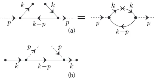
FIG. 1: Figure (a) depicts the cut diagram (left) and Feynman diagram (right) for the distribution functionfqπ(x). Solid lines denote the quark and dashed lines the pion. Herek−=x p− and the two quark lines with momentumk are connected by a γ+. Figure (b) depicts the cut diagram for the fragmentation function dπq(z). Herep− =z k−and the two quark lines with momentumk are connected by aγ+. This diagram refers to a frame where pT = 0 and the substitution given in Eq. (6) is performed in the final transverse momentum integral.
III. ELEMENTARY DISTRIBUTION AND FRAGMENTATION FUNCTIONS
The elementary distribution and fragmentation functions for the pion are represented in Figs. 1 as cut diagrams.
Since the distribution function can also be obtained from a straightforward Feynman diagram calculation [22, 30],6 we also illustrate the Feynman diagram for the distribution function on the right hand side in Fig. 1a. We denote the elementary fragmentation function by dhq in order to distinguish it from the total fragmentation function Dhq determined in Section IV. We obtain the following expressions from the diagrams in Figs. 1:7
fqπ(x) =1
2(1 +τπτq) 3gπ2
Z d4k (2π)4TrD
SF(k)γ+SF(k)γ5 k/−/p−M γ5
δ(k−−p−x)δ (p−k)2−M2
, (13)
=1
2(1 +τπτq) 6gπ2
Z d2kT
(2π)3
k2T+M2
k2T +M2−m2πx(1−x)2, (14) dπq(z) =1
2(1 +τπτq)g2πz 2
Z d4k (2π)4TrD
SF(k)γ+SF(k)γ5 k/−/p−M γ5
δ(k−−p−/z)δ (p−k)2−M2
, (15)
=z 6fqπ
x= 1
z
, (16)
=1
2(1 +τπτq)z g2π
Z d2p⊥ (2π)3
p2
⊥+M2z2
[p2⊥+M2z2+ (1−z)m2π]2, (17)
where TrD indicates a trace over Dirac indices only. The Feynman propagator of a constituent quark with mass M is denoted bySF and gπ is the pion-quark coupling constant. In the NJL model gπ is defined via the residue of the q¯q t-matrix at the pion pole, and can be expressed in terms of theqq¯bubble graph by
gπ−2=−∂Ππ(q2)
∂q2 q2=m2π
, where Ππ(q2) = 6i
Z d4k
(2π)4TrD[γ5SF(k)γ5SF(k+q)]. (18) We use the isospin notations (τu, τd) = (1,−1) and (τπ+, τπ0, τπ−) = (1,0,−1). For the distribution function in the physical region (0 < x < 1) a factor Θ (p−−k−) = Θ(1−x) has to be supplied in Eq. (13), which expresses the
6 This is seen simply by using completeness in Eq. (1) and the identityψ+(0)†ψ+(ω−) =T`
ψ+(0)†ψ+(ω−)´
in the limitω+ →0−ǫ, which follows from causality.
7 The expressions given in this section refer to the NJL model, however they actually have the same form in any effective chiral quark model with point-like pion-quark vertex functions.
FIG. 2: The quark self-energy, Σ(π)Q (k) =−3igπ2
R d4p
(2π)4γ5SF(k−p)γ5∆F(p), where ∆F is the Feynman propagator of the pion.
fact that the intermediate antiquark in Fig. 1a has positive energy. Similarly, for the fragmentation function a factor Θ(k−−p−) = Θ(1−z) has to be supplied in Eq. (15), because the intermediate quark in Fig. 1b has positive energy.
To obtain Eq. (17) we made the substitution given in Eq. (6).
The DLY relation on this level, indicated in brackets as Eq. (16), shows that Eq. (13) can be considered as a generalized distribution function, which gives the physical distribution function in the region 0 < x < 1 and the fragmentation function in the regionx= 1/z >1. The reason why we indicate this relation only in brackets is that it is violated if the integrals are regularized. For example, if we use a sharp cut-off (Λ) for the transverse quark momentum in Eq. (14), a strict application of the DLY relation would mean that the transverse momentum of the produced pion in Eq. (17) should be cut atzΛ, which is unacceptable. The more physical procedure is to impose
|kT|<Λ on Eq. (14) and|p⊥|<Λ on Eq. (17), which breaks the DLY relation. A similar breakdown of the DLY relation occurs in any other sensible regularization scheme. A noticeable consequence of this is that in the chiral limit the distribution function of Eq. (14) becomes a constant, but the fragmentation function of Eq. (17) is not linear in z, as the DLY relation indicated in Eq. (16) would suggest.
The relations for the distribution function Z 1
0
dx fqπ(x) = 1
2(1 +τπτq), and
Z 1 0
dx x fqπ(x) =1
2(1 +τπτq)· 1
2, (19)
lead to the usual number and momentum sum rules. For the elementary fragmentation function the following relation is obtained from Eq. (17):
Z 1 0
dz dπq(z) = 1
3(1 +τπτq) (1−ZQ) =⇒ Z 1
0
dz X
τπ
dπq(z) = 1−ZQ, (20) where ZQ is the residue of the quark propagator in the presence of the pion cloud. It is expressed in terms of the renormalized quark self-energy Σ(π)Q (k) of Fig. 2 as
1−ZQ=− ∂Σ(π)Q
∂/k
!
/ k=M
=−M
k− u¯Q(k)∂Σ(π)Q
∂k+
uQ(k)
!
= 3 2gπ2
Z 1 0
z dz
Z d2p⊥ (2π)3
p2⊥+M2z2
[p2⊥+M2z2+ (1−z)m2π]2, (21) where uQ is the quark spinor (¯uQuQ = 1). BecauseZQ is interpreted as the probability to find abare constituent quark without the pion cloud, Eq. (20) indicates that the elementary fragmentation function is normalized to the number of pions per quark. This is expected from our general discussions in Section II and will be elucidated further below. Because typical values of ZQ in models based on constituent quarks are between 0.8 and 0.9, we see from Eq. (20) that the momentum sum rule R1
0 dz zP
τπ dπq(z) will be much smaller than typical empirical values. For example, the NLO analysis of Ref. [11] found a momentum sum of ≃ 0.74. From this we can anticipate that the elementary fragmentation functions,dπq, will be very small compared to the empirical ones (see Section V).
In order to confirm that this does not mean that momentum conservation is violated, we also give the expressions for the distribution function of a quark q inside a parent quark Q and for the fragmentation function of q → Q.
The operator definitions of these functions (fqQ(x) andDqQ(z)) are exactly the same as in Eqs.(1) and (2) with the replacementh→Q, where the state|p(Q)irefers to fixed flavour, spin and color (c.f. the comments in footnote 3).
Again we will use the symbol dQq to denote the elementary fragmentation process. The relevant cut diagrams are
FIG. 3: Figure (a) depicts the cut diagram (left) and Feynman diagram (right) for the loop term in fqQ(x) of Eq. (22). Here k−=x p−and the two quark lines with momentumkare connected by aγ+. Figure (b) depicts the cut diagram for the loop term indQq(z) of Eq. (23). Herep−=z k−and the two quark lines with momentum kare connected by aγ+. This diagram refers to a frame wherepT = 0 and the substitution in Eq. (6) is performed in the final transverse momentum integral.
shown in Fig. 3 and a straightforward calculation, following the rules already indicated in Eqs. (13) and (15), gives8 fqQ(x) =ZQδ(x−1)δq,Q+
1
2−τqτQ
6 3
2gπ2(1−x)
Z d2kT
(2π)3
k2T+M2(1−x)2
k2T +M2(1−x)2+x m2π2, (22) dQq(z) = 1
6ZQδ(z−1)δq,Q+1 6
1
2 −τqτQ
6 3
2gπ2(1−z)
Z d2p⊥ (2π)3
p2⊥+M2(1−z)2
[p2⊥+M2(1−z)2+z m2π]2. (23) In accordance with Eq. (8) these relations show that
dQq(z) = 1
6fqQ(z) =1
6fQq(z). (24)
Therefore the two quantities in Eqs. (22) and (23) describe essentially the same object, namely the splitting function of a quark to another quark, which also includes a “non-splitting” term proportional toZQ. The normalization is
Z 1 0
dz6X
τQ
dQq(z) =ZQ+ (1−ZQ) = 1, (25)
where the factor 6 represents the summation over the spin and color ofQ. As expected, the second term in Eq. (23) can be obtained from the elementary q → π fragmentation function expressed in Eq. (17), via the substitutions z→1−zandτπ→(τq−τQ)/2. This directly leads to momentum conservation for the fragmentation ofqinto either Qorπ(see Eq. (29)).
This connection between splitting functions can also be viewed another way: The second term in Eq. (22), which describes the distribution ofq inside Qwith a pion spectator, suggests that via the substitutions τq/2→τQ/2−τπ
andx→1−xwe obtain the distribution function of a pion inside the quarkQ, namely fπQ(x) =1
2(1 +τπτQ)g2πx
Z d2kT
(2π)3
k2T +M2x2
k2T +M2x2+ (1−x)m2π2. (26)
8 The tree level terms proportional toZQin Eqs. (22) and (23) come from the vacuum state in the sum overnin Eqs. (1) and (2), which contributes for the case wherep(h) is a quark. Usingψ=p
ZQψ, where ˆˆ ψis the renormalized quark field with unit pole residue of the propagator, gives theZQterms in Eqs. (22) and (23). Note, in the loop terms all factorsZQof the propagators cancel. We also note that the loop terms infqQ(x) anddQq(z) formally satisfy the DLY relation, that is dQq,loop(z) = (−z/6)fq,loopQ (x= 1/z), however it is violated after regularization.
Comparison with Eq. (17) gives dπq(z) = fπq(z), in accordance with Eq. (8). This relation further elucidates the interpretation of the normalization given in Eq. (20) as the number of pions per quark, namely
Z 1 0
dz X
τπ
dπq(z) = Z 1
0
dz X
τπ
fπq(z) = 1−ZQ. (27)
Finally, we write down the momentum sum rules for the elementary splitting functions. In terms of the distribution functions we have
Z 1 0
dx x
X
τq
fqQ(x) +X
τπ
fπQ(x)
=ZQ+ Z 1
0
dx xX
τπ
fπQ(1−x) + Z 1
0
dx xX
τπ
fπQ(x) = 1, (28)
where in the second equality we used x → 1−x and Eq. (27). In terms of the fragmentation functions Eq. (28) becomes
Z 1 0
dz z
6X
τQ
dQq(z) +X
τπ
dπq(z)
= 1. (29) In reference to the form of Eq. (23), we have the following simple interpretation of the momentum sum rule of Eq. (29):
Because ZQ is the probability that the initial quark q does not fragment at all, the fraction ZQ of the momentum stays with the initial quark. The remaining fraction (1−ZQ) is shared among the quark remainder and the produced pion, that is, the first and second terms in Eq. (29).
Although a description of fragmentation functions using only the elementary fragmentation processes does not violate any conservation law, it is completely inadequate for the following reasons: Firstly, there is a large probability (ZQ) that the initial quark does not fragment. Secondly, if it does fragment the momentum fraction 1−ZQ is shared between the quark remainder and the pion. Both points are in contradiction to the usual assumption of complete hadronization, which is expressed by the momentum sum rule of Eq. (10).
IV. GENERALIZED PRODUCT ANSATZ FOR QUARK CASCADES
From the previous section, it is clear that we have to consider the possibility that the fragmenting quark produces a cascade of mesons. A simple model to describe cascades is the quark jet-model of Field and Feynman [19]. However, the product ansatz used in this model assumes from the outset that the probability for fragmentation in each elementary process is 100%, and that the quark produces an infinite number of mesons. Because these assumptions are inconsistent with our present effective quark theory, we will first introduce a generalized product ansatz, then explain its physical significance and its relation to the original quark jet-model.
We assume that the maximum number of mesons which can be produced by the fragmenting quark is N. We then consider a process where the initial quark with light-cone momentum k− ≡W0 (which we will simply call the momentum in the following) goes through a sequence of momentaW0 >W1 >W2>· · · >WN, and introduce the momentum ratios
ηn= Wn
Wn−1
, n= 1, . . . N. (30)
Our product ansatz for the fragmentation function, which we will motivate shortly, is:
Dqπ(z) =
N
X
m=1
Z 1 0
dη1
Z 1 0
dη2. . . Z 1
0
dηN
X
QN
6dQq1(η1)·6dQQ21(η2)· · · · ·6dQQN
N−1(ηN)δ(z−zm)δ τπ, τQm−1−τQm
/2 . (31)
Here the functionsdQQ′(η) are our elementaryQ→Q′ splitting functions of Eq. (23), which represent the probability that a quark of flavourQmakes a transition to the quarkQ′, leaving the momentum fraction η to Q′. A sum over repeated flavour indices is implied in Eq. (31); a flavour sum over the quark remainder (QN) is included; for the case N = 1 we define Q0 ≡ q; and the symbol δ(i, j) denotes the Kronecker delta. The factor 6 which multiplies each
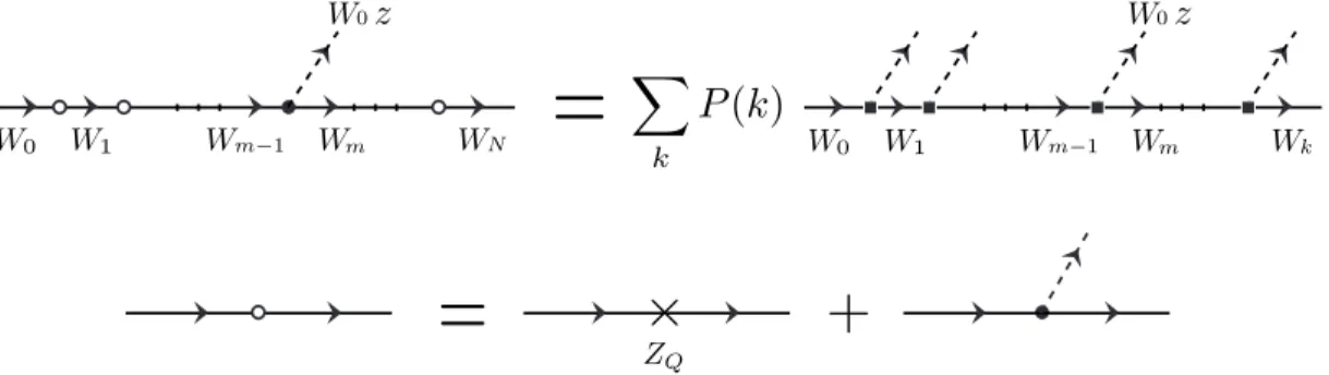
FIG. 4: The left hand side of the top figure is a graphical representation of Eq. (31) and the right hand side of this figure represents Eq. (37). The open circles denote the elementaryq→Qfragmentation function of Eq. (33) and the dots represent the second (meson emission) term in Eq. (33). In the mth step, where a meson with momentum z W0 is selected by the delta-function in Eq. (31), only the meson emission term contributes. The termP(k) is the binomial distribution of Eq. (38) and the squares represent the renormalized meson emission term, ˆFqQ(z), given by Eq. (40). The bottom figure is a graphical representaion of Eq. (33).
elementary splitting function comes from the sum over spin and color. The delta function in Eq. (31) selects a meson, which is produced in themth step with momentum fractionzmof the initial quark:
zm= Wm−1−Wm
W0 =η1·η2· · · · ·ηm−1·(1−ηm), where m >1, and z1= 1−η1. (32) Because the pion has a mass we will exclude the unphysical case ofz= 0, that is, whenever a pion is produced in the mth step we will assume thatηm6= 1 in Eq. (32).
We will write theq→Qsplitting function of Eq. (23), including the spin-color factor 6, in the form
6dQq(z) =ZQδ(z−1)δq,Q+FqQ(z), (33) where
FqQ(z) = 1
2 −τqτQ
6
F(z), and F(z) = 3
2g2π(1−z)
Z d2p⊥ (2π)3
p2⊥+M2(1−z)2 [p2
⊥+M2(1−z)2+z m2π]2. (34) The functionF satisfies the normalization (see Eq. (25))
X
Q
Z 1 0
dz FqQ(z) = Z 1
0
dz F(z) = 1−ZQ. (35)
For the case N = 1 it is easy to see that Eq. (31) reduces to the elementary fragmentation function of Eq. (17), namely
Dπq(z)N−→=1FqQ(1−z)|τQ=τq−2τπ = 1
3(1 +τqτπ)F(1−z) =dπq(z). (36) In order to illustrate the physical content of the ansatz expressed by Eq. (31) we rewrite it identically as follows:
Noting that each factor of the product in Eq. (31) consists of the two terms in Eq. (33), it is easy to see that all products with the same number (call itk) ofF′sand (N−k) number ofZQ’s make the same contribution toDπq(z). Therefore we can introduce an ordering of theη’s in Eq. (31). That is, take the firstk η’s not equal to one (η1, η2, . . . ηk 6= 1), and the remainingη’s equal to one (ηk+1, ηk+2, . . . ηN = 1), multiply by the combinatoric factor Nk
and perform a sum overk. For some fixedk, only terms withm6kwill contribute to the sum in Eq. (31), becausezmof Eq. (32)
must be non-zero.9 Then Eq. (31) is rewritten identically as Dqπ(z) =
N
X
m=1 N
X
k=m
P(k) Z 1
0
dη1
Z 1 0
dη2. . . Z 1
0
dηk
X
Qk
FˆqQ1(η1) ˆFQQ12(η2). . .FˆQQkk
−1(ηk)δ(z−zm)δ τπ, τQm−1−τQm
/2 ,
≡
N
X
m=1
Dπq,(m)(z), (37)
which is expressed graphically in Fig 4. The binomial distribution P(k) =
N k
ZQN−k(1−ZQ)k, (38)
is the probability of producingk mesons out of a maximum ofN mesons and satisfies the normalization condition
N
X
k=0
P(k) = 1. (39)
In Eq. (37) we defined the renormalized function ˆFqQ≡FqQ/(1−ZQ), that is (see Eqs. (34) and (35)) FˆqQ(z) =
1
2−τqτQ
6
Fˆ(z), where Fˆ(z) = F(z)
1−ZQ, and (40)
Z 1 0
dz X
Q
FˆqQ(z) = Z 1
0
dzFˆ(z) = 1. (41)
The physical interpretation of Eq. (37) is as follows:
• P(k) is the probability thatk mesons out of a maximum ofN mesons are produced.
• FˆQQ′(η) is the probability density that,if a meson is emitted from the quarkQ, the momentum fractionηis left to the remaining quarkQ′.
• The product ˆF(η1)·Fˆ(η2). . .F(ηˆ k) is the probability density that,if kmesons are produced, each meson carries its momentum fractionzm(m= 1, . . . k) of the original quark, where zmis given by Eq. (32).
• Dπq,(m)(z) is the probability density that the mth meson has the momentum fraction z of the original quark.
This implies that at least m mesons must be produced, which corresponds to the lower limit (k= m) of the summation in Eq. (37). The total fragmentation function Dqπ(z) is then obtained by summing the probability densitiesDπq,(m)(z).
We note that the original ansatz of Field and Feynman [19] is an infinite product, which formally emerges from Eq. (37) if we take the limitN → ∞and assume thatP(k) is equal to zero for any finite k, that is, the probability of the fragmenting quark to emit a finite number of mesons is zero.
We now proceed with Eq. (37) in order to find the integral equation satisfied by the fragmentation function. For a fixedm, we can integrate overηm+1, . . . ηN by using the normalization of ˆF, that is,
Z 1 0
dηX
Q
FˆqQ(η) = Z 1
0
dη Z 1
0
dη′ X
Q′
FˆqQ(η) ˆFQQ′(η′) =· · ·= 1. (42)
9 As explained earlier, we only consider the casez >0.
dˆπq(z) = ˆFqQ(1−z)|τQ=τq−2τπ = 1
3(1 +τqτπ) ˆF(1−z). (44) From Eq. (43) it is easy to derive the following recursion relation form >1:
Dq(m)π (z) =Rm
hFˆqQ⊗DπQ(m−1)i
(z), where m >1, (45)
while form= 1 we have
Dπq(1)(z) =R1dˆπq(z). (46)
We have introduced the following ratios:
Rn= PN
k=nP(k) PN
k=n−1P(k), where n= 1,2, . . . N, (47)
and used the following notation for the convolution of two functionsA(z) andB(z):
[A⊗B] (z) = Z 1
0
dz1
Z 1 0
dz2δ(z−z1z2)A(z1)B(z2). (48) The total fragmentation function then becomes
Dqπ(z) =R1dˆπq(z) +
N
X
n=2
Rn
hFˆqQ⊗DπQ(n−1)i
(z), (49)
whereDπq(m)can be obtained from the recursion relation of Eq. (45), with the starting value given by Eq. (46).
It is interesting at this stage to derive the sum rules for the fragmentation function. A simple calculation using Eq. (43) gives the following expressions for the multiplicity, the momentum sum and the isospin sum:
Z 1 0
dzX
τπ
Dqπ(z) =
N
X
k=1
kP(k) =N(1−ZQ), (50)
Z 1 0
dzX
τπ
z Dqπ(z) = 1−
N
X
k=0
P(k)hzFˆik = 1−
ZQ+ (1−ZQ)hzFˆiN
, (51)
Z 1 0
dzX
τπ
τπDqπ(z) = τq
2
"
1−
N
X
k=0
P(k)
−1 3
k#
=τq
2
"
1−
ZQ−1
3(1−ZQ) N#
, (52)
wherehAi ≡R1
0 dzA(z). These expressions can be understood as follows: If kmesons are produced with probability P(k), then Eq. (50) is simply the mean number of mesons; the quantityP(k)hzFˆikin Eq. (51) is the mean momentum fraction left to the quark remainder; and the quantityP(k) (−1/3)k in Eq. (52) is the mean isospin fraction left to the quark remainder.
Eqs. (51) and (52) indicate that, in the present model, it is not possible to transfer the total momentum and isospin of the original quark to the mesons, if the maximum number of mesons is finite. The momentum and isospin sum rules given in Eqs. (10) and (11) are valid only in the limitN → ∞. While this may indicate a conceptual limitation
of the jet-model, we note that in general, the QCD based empirical analysis of fragmentation functions also leads to divergent multiplicities. Therefore, we find it more important to satisfy the momentum and isospin sum rules given in Eqs. (10) and (11) than to have finite multiplicities, and therefore we take the limitN → ∞. The results then become independent of the form of the distributionP(k), if the following condition is satisfied for the ratios in Eq. (47):
Rn N→∞
−→ 1, for all n= 1,2, . . . (53)
In fact, it is well known that in the limit N → ∞ our binomial distribution of Eq. (38) becomes a normalized Gaussian distribution (normal distribution) √1
2πc2e−(k−k0 )
2
2c2 , with the same mean valuek0=N(1−ZQ) and variance c2 =N ZQ(1−ZQ) as the original binomial distribution. The validity of Eq. (53) can then easily be confirmed. In fact, any distribution which approaches a normal distribution in the limitN → ∞satisfies the condition given in Eq. (53).10
Using Eq. (53), we see from Eq. (49) that our fragmentation function satisfies essentially the same integral equation as in the original quark jet-model [19]:
Dqπ(z) = ˆdπq(z) +h
FˆqQ⊗DπQi
(z), (54)
where the driving term is given by Eq. (44) and the integral kernel by Eq. (40). We finally write down the equations which we solve in the next section. Defining two functionsA(z) andB(z) by the isospin decomposition
Dqπ(z)≡ 1
3[A(z) +τqτπB(z)], (55)
and using Eqs. (40) and (44), we find the following integral equations forA(z) andB(z) from Eq. (54):
A(z) = ˆF(1−z) + Z 1
z
dy y Fˆ
z y
A(y), (56)
B(z) = ˆF(1−z)−1 3
Z 1 z
dy y Fˆ
z y
B(y), (57)
where ˆF(z) is obtained by renormalizing the functionF(z) in Eq. (34) to unity. Using Eq. (55), we obtain the following expressions for the favoured, unfavoured andneutral fragmentation functions:
Dπu+=Ddπ− =Dπu¯− =Dπd¯+ =1
3(A+B), (58)
Dπu− =Ddπ+=Dπ¯u+ =Dπd¯−= 1
3(A−B), (59)
Dπu0 =Ddπ0 =Dπu¯0=Dπd¯0 = 1
3A. (60)
From the form of Eqs. (56) and (57) it is easily seen thathz Ai= 1 andhBi= 3/4, which leads to the momentum and isospin sum rules of Eqs. (10) and (11). For largez, both functionsA(z) andB(z) approach ˆF(1−z) and therefore the unfavored fragmentation functions in Eq. (59) are suppressed for large pion momenta.
V. NUMERICAL RESULTS AND DISCUSSIONS
In this section we present the numerical results for the fragmentation function of Eq. (54) in the NJL-jet model.
For reference, we also give the results for the elementary distribution function of Eq. (14). Because the application of the NJL model to the calculation of the quark distribution functions in the pion has been explained in detail in
10The fact that in the limitN → ∞the binomial distribution becomes a normal distribution is known as the Moivre-Laplace theorem, which can be formulated rigorously in integral form (“weak convergence”). The central limit theorem [31] is an extension of the Moivre- Laplace theorem to general distributionsP(k) with mean value proportional toNand variancec2∝N. This indicates that Eq. (53) is actually valid for a wide class of distributions. Although our NJL-jet model ansatz of Eq. (31) leads to the binomial distribution, in the limitN→ ∞the results hold for a wide class of distributions.
In terms of light-cone variables, if we associate with particle 1 the transverse momentum qT and the momentum fractiony of the totalP− momentum, and to particle 2 we associate the momentum fraction (1−y) and transverse momentum−qT, then their invariant mass squared is
M122 =M12+q2T
y +M22+q2T
1−y . (62)
The requirementM126Λ12 then leads to ay-dependent transverse cut-off: q2T 6Λ212y(1−y)−M12(1−y)−M22y.
This condition also restricts the values of y from below and above (0 < y1 6 y 6 y2 < 1). For example, for the integral in Eq. (17) of the elementaryq→πfragmentation function we haveM1=mπ andM2=M, for the integral in Eq. (23) of the elementaryq→Qfragmentation function we haveM1=M and M2=mπ and for the integral in Eq. (14) of the distribution function we haveM1=M2=M. We also note that this regularization scheme does not violate the sum rules.
Following Ref. [22] we use a constituent quark mass ofM = 300 MeV. Then Λ3= 670 MeV and the invariant mass cut-offs for the (π, q) and (q, q) systems are 1.42 GeV and 1.47 GeV, respectively. We did not investigate whether other parameter sets or other regularization schemes lead to a better description of the fragmentation functions.
As usual, we will associate a low energy renormalization scale (Q20) to our NJL results and evolve them inQ2 by using the QCD evolution equations. For the evolution of the fragmentation functions we limit ourselves to LO. In this case it has been verified [17] that a formal application of the DLY relation, see Eq. (12), leads to the correct connection between the evolution kernels of the distribution and fragmentation functions (see Appendix B). However, the DLY relation is not actually used to relate the distribution and fragmentation functions themselves. We therefore use the Q2 evolution code of Ref. [33] at LO for the distribution functions, and perform the transformation of the kernels as explained in Appendix B to obtain the LO evolution of the fragmentation functions.11
In Fig. 5a we recapitulate the results of Fig. 4 of Ref. [22], and show the minus-type (valence, q−q)¯ u-quark distribution in aπ+ and in Fig. 5b we give the result for theplus-type (q+ ¯q) u-quark distribution in aπ+. The dotted line shows the NJL model result based on Eq. (14), the solid lines illustrate the distribution obtained by associating a low energy scale ofQ20= 0.18 GeV2 to the NJL result and performing theQ2evolution at LO and NLO to Q2 = 4 GeV2. The dashed line shows the empirical NLO parametrizations of Ref. [8]. We see that the LO and NLO results show quantitative differences because of the rather low value assumed for Q20, although the qualitative behaviours are similar.
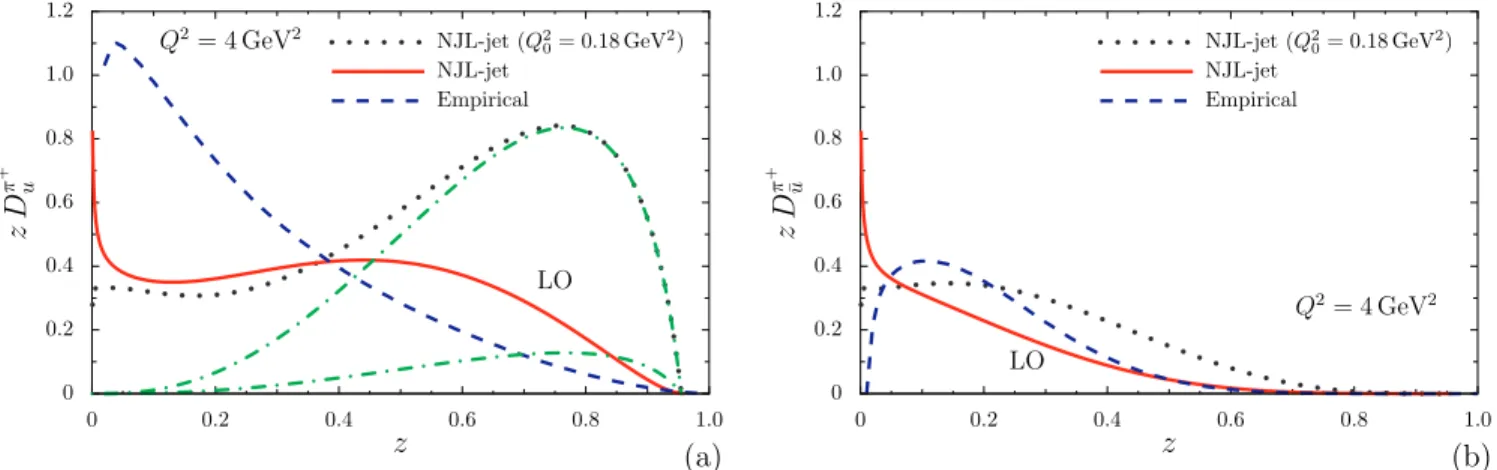
In Figs. 6 we present the corresponding results for the minus-type and plus-type fragmentation functions foru→π+. The NJL-jet result, given by the dotted line, is the solution of the integral equation in Eq. (54). Therefore the dotted line in Figs. 6a and 6b show the functions 23B(z) and 23A(z), respectively (see Eqs.(58) and (59)). In order to see the importance of the cascade processes, we also plot the driving term of the integral equation, namely 23Fˆ(1−z), as the upper dash-dotted line, which is the renormalized elementary fragmentation function. As the lower dash-dotted line we illustrate the elementary fragmentation function, namely 23F(1−z). The result of the evolution of the dotted line (Q20 = 0.18 GeV2) toQ2 = 4 GeV2 at LO is shown by the solid line and the dashed line shows the empirical NLO result of Ref. [11], evolved toQ2= 4 GeV2.
Several important points are illustrated in Figs. 6. Firstly, as anticipated in Section III, the elementary frag- mentation function (lower dash-dotted line) is very small. Secondly, Fig. 6b shows the tremendous enhancement at intermediate and smallz of the plus-type fragmentation function caused by the cascade processes (iterations of the integral equation of Eq. (54)), while for the minus-type fragmentation function of Fig. 6a a small reduction is seen.
11The DLY based relation between the evolution kernels for distribution and fragmentation functions is violated at NLO [17]. Unfortu- nately, a NLO evolution code for the fragmentation functions is not yet publicly available. In this paper we do not attempt a quantitative comparison with the empirical functions, therefore we leave the NLO calculation for future work.