Complex Phase Pattern in Chaotic Circuits with Time-Varying Resistors

(1)

社団法人電子情報通信学会

THE INSTITUTE OF ELECTRONICS,

INFORMATION AND COMMUNICATION ENGINEERS

信学技報

TECHNICAL REPORT OF IEICE.

時変抵抗で結合されたカオス回路で観測される複雑位相パターンについて

上手洋子

^†

西尾芳文

^††

ルディストープ

^†

†Institute of Neuroinformatics, University / ETH Zurich CH-8057 Winterthurerstrasse 190, Zurich, Switzerland

††徳島大学大学院ソシオテクノサイエンス研究部

〒770–8506徳島市南常三島2–1

E-mail: †{yu001,ruedi}@ini.phys.ethz.ch,††[email protected]

あらまし近年、カオス結合系で観測される位相同期現象についての調査が活発に行われている。このような結合系は様々な種類の位相パターンを生み出すことが知られており、この位相パターンを連想記憶や学習過程のモデリングに応用できるのではないかと期待されている。本研究では、リング状に時変抵抗で結合したカオス回路で観測される同期現象について調査を行う。コンピュータシミュレーションの結果、van der Pol発振器で観測された位相伝搬派とは異なる複雑位相パターンを観測することができた。さらに、観測された複雑位相パターンの評価方法として、時間空間エントロピーを適用した。

キーワード結合発振器，複雑位相パターン，時変抵抗

Complex Phase Pattern in Chaotic Circuits with Time-Varying Resistors

Yoko UWATE^†, Yoshifumi NISHIO^††, and Ruedi STOOP^†

† University / ETH Zurich CH-8057 Winterthurerstrasse 190, Zurich, Switzerland

††Tokushima University 2–1 Minami Josanjima, Tokushima, 770–8506 Japan E-mail: †{yu001,ruedi}@ini.phys.ethz.ch,††[email protected]

Abstract Recently, studies on phase synchronization phenomena of coupled chaotic oscillators are extensively carried out by many researchers. Such oscillatory systems can produce some kinds of phase patterns, and they may be utilized modeling for associative memory and learning process. In this study, we investigate the synchronization phenomena in chaotic circuits coupled by time-varying resistor as a ring. By carrying out computer simulations, we conﬁrm the complex phase pattern which cannot be observed in simple oscillatory systems coupled by a resistor.

Furthermore, we apply a space-time entropy to evaluate complex phase patterns obtained form coupled chaotic circuits.

Key words coupled oscillators, complex phase pattern, time-varying resistor

1. Introduction

Recently, studies on phase synchronization phenomena of coupled chaotic oscillators are extensively carried out by many researchers [1]- [9]. Such oscillatory systems can produce some kinds of phase patterns, and they may be utilized modeling for associative memory and learning process. Endo et al. have reported details of theoretical analysis and circuit experiments about some coupled oscillators as a ladder, a

ring and a two-dimensional array [10]. Yamauchi et al. have discovered very interesting wave propagation phenomena of phase states between two adjacent oscillators in an array of van der Pol oscillators coupled by inductors [11].

On the other hand, there are some systems whose dissi- pation factors vary with time, for example, under the time- variation of the ambient temperature, an equation describing an object moving in a space with some friction and an equation governing a circuit with a resistor whose temperature

(2)

x1+x2 x2+x3 x3+x4 x4+x5 x5+x6 x6+x7 x7+x8 x8+x9 x9+x10 x11+x12 x12+x13 x13+x14 x14+x15 x15+x1 x10+x11

τ (a) Wave extinction.

τ (b) Random pattern.

τ (c) Wave propagation.

τ (d) Clusterling.

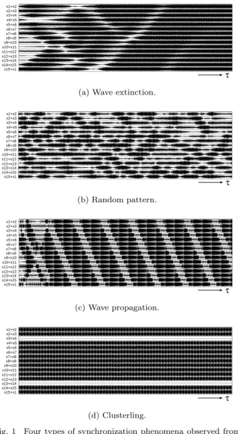
Fig. 1 Four types of synchronization phenomena observed from a ring of van der Pol oscillators coupled by time varying resistors.

2L1

2L1 2L1 2L1

TVR C

vd(ik)

TVR TVR

L2

-r vk

ILk IRk IL(k+1)IR(k+1)

ik

C

vd(ik+1) L2

-r vk+1

ik+1

Fig. 2 Coupled oscillators model.

coeﬃcient is sensitive such as thermistor. However, there are few discussion about coupled oscillators coupled by a time-varying resistor.

In our previous research, we have investigated the synchronization phenomena in van der Pol oscillators coupled by time-varying resistor as a ring [12], [13]. We realized the time-varying resistor by switching a positive and a negative resistor periodically. We conﬁrmed the various interesting phenomena (wave extinction, randam pattern, wave propa-

gation and clustering) as shown in Fig. 1.

In this study, we investigate the complex phase pattern when coupled van der Pol oscillator is changed to chaotic circuit. First, the case of even number coupling, the coexistence of in-phase and anti-phase states are observed. In con- trast, the case of odd number coupling, we can conﬁrm the coexistence between in-phase and n-phase states. Second, the coexistence area changing the bifurcation parameter of chaotic circuits is investigated. By carrying out computer simulations, we conﬁrm the complex phase pattern which cannot be observed in simple oscillatory systems coupled by a resistor. Next, we apply a space-time entropy to evaluate complex phase patterns obtained form coupled chaotic circuits.

2. Coupled Oscillators Model

In this study, we consider a ring of chaotic circuits as shown in Fig. 2. In this circuit adjacent two chaotic circuits are coupled by one time-varying resistor (TVR). We realize the TVR by switching a positive and a negative resistors periodically as shown in Fig. 3.

2πp 2π R(t)

ω^tt

0

r

-r

Fig. 3 Characteristics of the TVR.

First, the i−v characteristics of the diode are approxi- mated by two-segment piecewise linear function as

vd(ik) =1

2(rdik+E− |rdik−E|). (1) By changing the variables and the parameters,

IRk =

√C L1

ExRk, ILk=

√C L1

ExLk, ik=

√C L1

Eyk,

vk=Ezk, t=√ L1Cτ ,

α= L1

L2

, β=r

√C L1

, γ=R

√C L1

, δ=rd

√C L1

,

ω= 1

√L1Cωτ,

the normalized circuit equations of the ring of chaotic circuits are given as

(3)









 dxRk

dτ =1

2{β(xRk+xLk+yk)−zk−γ(xRk+xL(k+1))}

dxLk

dτ =1

2{β(xRk+xLk+yk)−zk−γ(xLk+xL(R+1))}

dyk

dτ =α{β(xRk+xLk+yk)−zk−f(yk)} dzk

dτ =xRk+xLk+yk

(k= 1,2,3,· · ·, N)

(2)

where f(yk) =1

2(δyk+ 1− |δyk−1|) (3) and

xLN =xL1, xR0=xRN. (4) It should be noted that γ corresponds to the coupling strength and that β corresponds to the bifurcation parameter of chaotic circuits. Eq. (2) is calculated by using the fourth-order Runge-Kutta method.

3. Synchronization Phenomena

3. 1 Even Number Coupling:N = 14

Figure 4 shows the computer simulated result for the case ofN= 14. Ndenotes the number of coupled oscillators. We can see that the ring of chaotic circuits coupled by TVR are synchronized at in-phase or at anti-phase.

3. 2 Odd Number Coupling:N = 15

Figure 5 shows the computer simulated result for the case ofN= 15. We also can see that the ring of chaotic oscillators coupled by TVR are synchronized with in-phase (Fig. 5(a)).

And the adjacent circuts are almost synchronized with anti- phase as shown in Fig. 5(b). Because, the boundary condi- tion is the ring structure, the phase diﬀerence between the adjacent circuits is not around π. Namely, in this case 15- phase synchronization are observed.

3. 3 Complex Phase Patterns

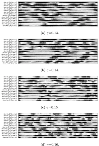
Here, we investigate the synchronization phenomena when the strength of the coupling parameter γ is decreased. We ﬁnd complex phase patterns as shown in Figs. 6-7. These phenomena can be observed by switching of the phase states between the in-phase and the anti-phase synchronization with two adjacent chaotic circuits, whereas the white region shows the in-phase synchronization. From these ﬁgures, the wave of the anti-phase propagates without regular rule.

Figures 8-9 show the coupling strength of breakdown synchronization from coexistence to phase pattern phenomena by changing the bifurcation parameter βof the chaotic circuit. We conﬁrm that the coupling strength of breakdown of synchronization becomes large by increasing bifurcation

(a) In-phase synchronization.

(b) Anti-phase synchronization.

Fig. 4 Computer simulated result forN = 14. α = 7.0, β = 0.094, δ = 50.0, ω = 1.924, γ = (0.2 or −0.2). Up- per ﬁgures:xRk+xLkvszk. Middle ﬁgures:xRk+xLk

vs x_R(k+1)+x_L(k+1). Lower ﬁgures: τ vs xRk+xLk. k= 1,2,3, . . . ,14.

Attractor Phase difference

xR1+xL1 xR2+xL2 xR3+xL3 xR4+xL4 xR5+xL5 xR6+xL6 xR7+xL7 xR8+xL8 xR9+xL9 xR10+xL10 xR11+xL11 xR12+xL12 xR13+xL13 xR14+xL14

τ

xR15+xL15

(a) In-phase synchronization.

Attractor Phase difference

xR1+xL1 xR2+xL2 xR3+xL3 xR4+xL4 xR5+xL5 xR6+xL6 xR7+xL7 xR8+xL8 xR9+xL9 xR10+xL10 xR11+xL11 xR12+xL12 xR13+xL13 xR14+xL14

τ

xR15+xL15

(b) 15-phase synchronization.

Fig. 5 Computer simulated result forN = 15. α = 7.0, β = 0.094, δ = 50.0, ω = 1.924, γ = (0.2 or −0.2). Up- per ﬁgures:xRk+xLkvszk. Middle ﬁgures:xRk+xLk

vs x_R(k+1)+x_L(k+1). Lower ﬁgures: τ vs xRk+xLk. k= 1,2,3, . . . ,15.

parameterβ.

The examples of complex phase pattern are shown in Figs. 10-11 when the parameterβandγ are changed.

(4)

Fig. 6 Complex phase pattern for N = 14. α = 7.0, β = 0.094,δ= 50.0,ω= 1.924,γ= (0.166 or−0.166).

(x^R1+x^L1)+(x^R2+x^L2) (xR2+xL2)+(xR3+xL3) (xR3+xL3)+(xR4+xL4) (xR4+xL4)+(xR5+xL5) (xR5+xL5)+(xR6+xL6) (xR6+xL6)+(xR7+xL7) (xR7+xL7)+(xR8+xL8) (xR8+xL8)+(xR9+xL9) (xR9+xL9)+(xR10+xL10) (x^R10+x^L10)+(x^R11+x^L11) (xR11+xL11)+(xR12+xL12) (xR12+xL12)+(xR13+xL13) (xR13+xL13)+(xR14+xL14)

τ

(xR15+xL15)+(xR1+xL1) (x^R14+x^L14)+(x^R15+x^L15)

Fig. 7 Complex phase pattern for N = 15. α = 7.0, β = 0.094,δ= 50.0,ω= 1.924,γ= (0.136 or−0.136).

0.06 0.065 0.07 0.075 0.08 0.085 0.09 0.095

0.13 0.135 0.14 0.145 0.15 0.155 0.16 0.165 0.17

β (bifurcation parameter)

γ (coupling strength) Coexistence

(in-phase & anti-phase) Switching: phase pattern

(in-phase & anti-phase)

Fig. 8 Synchronization types (N = 14). α= 7.0,δ= 50.0,ω= 1.924.

0.06 0.065 0.07 0.075 0.08 0.085 0.09 0.095

0.13 0.135 0.14 0.145 0.15 0.155 0.16 0.165 0.17 0.175

β (bifurcation parameter)

γ (coupling strength) Coexistence

(in-phase & 15-phase) Switching

(in-phase & 15-phase)

Fig. 9 Synchronization types (N = 15). α= 7.0,δ= 50.0,ω= 1.924.

4. Entropy

In order to capture the properties of cellular automata a space-time entropy have been introduced [16]. The space- time entropy of cellular automata with ncells is deﬁned as follows:

(xR1+xL1)+(xR2+xL2) (xR2+xL2)+(xR3+xL3) (xR3+xL3)+(xR4+xL4) (xR4+xL4)+(xR5+xL5) (xR5+xL5)+(xR6+xL6) (xR6+xL6)+(xR7+xL7) (xR7+xL7)+(xR8+xL8) (xR8+xL8)+(xR9+xL9) (xR9+xL9)+(xR10+xL10) (xR10+xL10)+(xR11+xL11) (xR11+xL11)+(xR12+xL12) (xR12+xL12)+(xR13+xL13) (x^R13+x^L13)+(x^R14+x^L14)

τ (xR15+xL15)+(xR1+xL1)

(xR14+xL14)+(xR15+xL15)

(a)β=0.065.

(x^R1+x^L1)+(x^R2+x^L2) (xR2+xL2)+(xR3+xL3) (xR3+xL3)+(xR4+xL4) (xR4+xL4)+(xR5+xL5) (xR5+xL5)+(xR6+xL6) (xR6+xL6)+(xR7+xL7) (xR7+xL7)+(xR8+xL8) (xR8+xL8)+(xR9+xL9) (xR9+xL9)+(xR10+xL10) (xR10+xL10)+(xR11+xL11) (xR11+xL11)+(xR12+xL12) (xR12+xL12)+(xR13+xL13) (xR13+xL13)+(xR14+xL14)

τ (xR15+xL15)+(xR1+xL1)

(xR14+xL14)+(xR15+xL15)

(b)β=0.075.

(x^R1+x^L1)+(x^R2+x^L2) (x^R2+x^L2)+(x^R3+x^L3) (xR3+xL3)+(xR4+xL4) (xR4+xL4)+(xR5+xL5) (xR5+xL5)+(xR6+xL6) (xR6+xL6)+(xR7+xL7) (xR7+xL7)+(xR8+xL8) (xR8+xL8)+(xR9+xL9) (xR9+xL9)+(xR10+xL10) (xR10+xL10)+(xR11+xL11) (xR11+xL11)+(xR12+xL12) (xR12+xL12)+(xR13+xL13) (xR13+xL13)+(xR14+xL14)

τ (xR15+xL15)+(xR1+xL1)

(xR14+xL14)+(xR15+xL15)

(c)β=0.085.

(xR1+xL1)+(xR2+xL2) (xR2+xL2)+(xR3+xL3) (x^R3+x^L3)+(x^R4+x^L4) (xR4+xL4)+(xR5+xL5) (xR5+xL5)+(xR6+xL6) (xR6+xL6)+(xR7+xL7) (xR7+xL7)+(xR8+xL8) (xR8+xL8)+(xR9+xL9) (xR9+xL9)+(xR10+xL10) (xR10+xL10)+(xR11+xL11) (xR11+xL11)+(xR12+xL12) (xR12+xL12)+(xR13+xL13) (xR13+xL13)+(xR14+xL14)

τ (xR15+xL15)+(xR1+xL1)

(xR14+xL14)+(xR15+xL15)

(d)β=0.095.

Fig. 10 Examples of pahse propagation by changing β from 0.065 to 0.095. α = 7.0, δ = 50.0, ω = 1.924,γ = (0.132 or−0.132).

S =−1 n

1 T

∑

i

∑

t

∑

m

c^t_i,m

∑

mc^t_i,mlog2

c^t_i,m

∑

mc^t_i,m (5) where ^c

t

∑i,m mc^t

i,m

denotes the probabilities and m counts the two possible statesai ∈ {0,1} of cell. This space-time entropy is a measure of the order some cellular automata conﬁguration at a number of cellnand a ﬁxed timeT(=65).

We apply the space-time entropy to evaluation of complex phase patterns obtained from a ring of chaotic circuits.

First, obtained complex phase patterns are changed to discrete pattern data like cellular automata. In order to distin- guish in-phase or anti-phase synchronization, the threshold valueth= 1.0 is introduced as shown in Fig. 12. Whenthis larger than 1.0, the synchronization state is anti-phase.

The discrete data patterns obtained from Figs. 10-11 are shown in Figs. 13-14. “¥(1)” and “¤(0)” are corresponding to the in-phase and the anti-phase synchronization, respec- tively. We caluculate the space-time entropy for these discrete pattern data and the value of entropy are described in subcaption of each ﬁgures. From these results, all entropies show high value which is larger than 0.9.

(5)

(xR1+xL1)+(xR2+xL2) (xR2+xL2)+(xR3+xL3) (xR3+xL3)+(xR4+xL4) (xR4+xL4)+(xR5+xL5) (xR5+xL5)+(xR6+xL6) (xR6+xL6)+(xR7+xL7) (x^R7+x^L7)+(x^R8+x^L8) (xR8+xL8)+(xR9+xL9) (xR9+xL9)+(xR10+xL10) (xR10+xL10)+(xR11+xL11) (xR11+xL11)+(xR12+xL12) (xR12+xL12)+(xR13+xL13) (xR13+xL13)+(xR14+xL14)

τ

(x^R15+x^L15)+(x^R1+x^L1) (xR14+xL14)+(xR15+xL15)

(a)γ=0.13.

(xR1+xL1)+(xR2+xL2) (x^R2+x^L2)+(x^R3+x^L3) (xR3+xL3)+(xR4+xL4) (xR4+xL4)+(xR5+xL5) (xR5+xL5)+(xR6+xL6) (x^R6+x^L6)+(x^R7+x^L7) (xR7+xL7)+(xR8+xL8) (xR8+xL8)+(xR9+xL9) (x^R9+x^L9)+(x^R10+x^L10) (xR10+xL10)+(xR11+xL11) (xR11+xL11)+(xR12+xL12) (xR12+xL12)+(xR13+xL13) (x^R13+x^L13)+(x^R14+x^L14)

τ

(xR15+xL15)+(xR1+xL1) (xR14+xL14)+(xR15+xL15)

(b)γ=0.14.

(x^R1+x^L1)+(x^R2+x^L2) (xR2+xL2)+(xR3+xL3) (xR3+xL3)+(xR4+xL4) (xR4+xL4)+(xR5+xL5) (xR5+xL5)+(xR6+xL6) (xR6+xL6)+(xR7+xL7) (xR7+xL7)+(xR8+xL8) (x^R8+x^L8)+(x^R9+x^L9) (xR9+xL9)+(xR10+xL10) (xR10+xL10)+(xR11+xL11) (xR11+xL11)+(xR12+xL12) (xR12+xL12)+(xR13+xL13) (xR13+xL13)+(xR14+xL14)

τ

(c)γ=0.15.

(xR1+xL1)+(xR2+xL2) (xR2+xL2)+(xR3+xL3) (x^R3+x^L3)+(x^R4+x^L4) (xR4+xL4)+(xR5+xL5) (xR5+xL5)+(xR6+xL6) (xR6+xL6)+(xR7+xL7) (x^R7+x^L7)+(x^R8+x^L8) (xR8+xL8)+(xR9+xL9) (xR9+xL9)+(xR10+xL10) (x^R10+x^L10)+(x^R11+x^L11) (xR11+xL11)+(xR12+xL12) (xR12+xL12)+(xR13+xL13) (xR13+xL13)+(xR14+xL14)

τ

(d)γ=0.16.

Fig. 11 Examples of pahse propagation by changingγfrom 0.13 to 0.16. α= 7.0,β=0.094,δ= 50.0,ω= 1.924.

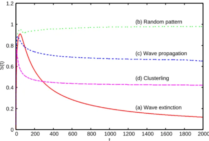
For comparison, we also apply the space-time entropy to complex phase patterns (Fig. 1) obtained from a ring of van der Pol oscillators. The discrete data of phase patterns and the value of the space-time entropy are shown in Fig. 15.

From these results, we conﬁrm that the space-time entropy of phase patterns obtained from chaotic circuits is higher value than the van der Pol oscillators.

Finally we caluculate the time evolution of average entropy and the obtained results are shown in Figs. 16, 17. In the case of the chaotic circuits (Fig. 16), the every average entropy show high value. While, in the case of the patterns obtained from the van der Pol oscillators, each pattern con- verge the diﬀerent entropy value. We consider that it is one possibility to classiﬁcate these complex patterns obtained the ring of van der Pol oscillators and chaotic circuits by using space-time entropy.

5. Conclusions

In this study, we have investigated synchronization phenomena in chaotic circuits coupled by time varying resistors as a ring. By computer simulations, ﬁrst we conﬁrmed the coexistence of in-phase and anti-phase synchronizations. Next,

-2 -1 0 1 2

0 20000 40000 60000 80000 100000 120000

(XR1+XL1)+(XR2+XL2)

τ

th=1.0

Fig. 12 Threshold for distinguishing in-phase or anti-phase synchronization.

(a)β=0.065,S=0.932.

(b)β=0.075,S=0.934.

(c)β=0.085,S=0.948.

(d)β=0.095,S=1.000.

Fig. 13 Discrete data obtained from Fig 10.

(a)γ=0.13,S=0.961.

(b)γ=0.14,S=0.974.

(c)γ=0.15,S=0.987

(d)γ=0.16,S=0.989.

when the coupling strength decreases, we observed complex phase pattern which cannot be observed in simple oscillatory circuits coupled by resistors. Furthermore, we appled the space-time entropy to evaluate complex phase patterns.

The space-time entropy obtained from the coupled chaotic oscillators showed high values have been observed.

(6)

(a)S=0.575.

(b)S=0.920.

(c)S=0.720

(d)S=0.447.

0 0.2 0.4 0.6 0.8 1 1.2

0 200 400 600 800 1000 1200 1400 1600 1800 2000

S(t)

t (a) γ=0.13

(b) γ=0.14

(d) γ=0.16

(c) γ=0.15

Fig. 16 Time evolution of average entropy for chaotic circuits.

0 0.2 0.4 0.6 0.8 1 1.2

0 200 400 600 800 1000 1200 1400 1600 1800 2000

S(t)

t

(a) Wave extinction (b) Random pattern

(c) Wave propagation

(d) Clusterling

Fig. 17 Time evolution of average entropy for van der Pol oscillators.

References

[1] M. G. Rosenblum, A. S. Pikovsky and J. Kurths, “Phase Synchronization of Chaotic Oscillators,” Physical Review Letters, vol.11, March. 1996.

[2] G. V. Osipov, A. S. Pikovsky, M. G. Rosenblum and J.

Kurths, “Phase Synchronization Eﬀects in a Lattice of Non- identical R¨ossler Oscillators,” Physical Review E, vol.55, no.3 March. 1997.

[3] M. G. Rosenblum, A. S. Pikovsky, and J. Kurths, “Phase Synchronization in Driven and CoupledChaotic Oscilla- tors,” IEEE Transactions on Circuits and Systems-I:, vol.44, no.10, October. 1997.

[4] A. S. Pikovsky, M. G. Rosenblum, G. V. Osipov, J. Kurths,

“Phase Synchronization of Chaotic Oscillators by External Driving,”Physica D, 104, pp. 219-238, 1997.

[5] M. G. Rosenblum, A. S. Pikovsky and J. Kurths, “Phase Synchronization of Chaotic Oscillators,” Physical Review Letters, vol.11, March. 1996.

[6] Z. Zheng, G. Hu and B. Hu, “Phase Slips and Phase Syn- chronization of Coupled Oscillators,”Physical Review Let- ters, vol. 81, no.24, December. 1998.

[7] E. H. Park, M. A. Zaks, and J. Kurths, “Phase Synchro- nization in the Forced Lorenz System,”Physical Review E, vol.60, no.6 December. 1999.

[8] C. Zhou, J. Kurths, I. Z. Kiss and J. Hudson, “Noise- Enhanced Phase Synchronization of Chaotic Oscillators,”

Physical Review Letters, vol.89, no.1, July. 2002.

[9] C. Zhou and J. Kurths, “Noise-Induced Phase Synchroniza- tion and Synchronization Transitions in Chaotic Oscilla- tors,”Physical Review Letters, vol.88, no.23 June. 2002.

[10] T. Endo and S. Mori, “Mode Analysis of a Ring of a Large Number of Mutually Coupled van der Pol Oscilla- tors,”IEEE Trans. Circuits Systems, vol.25, no.1, pp.7-18, Jan. 1978.

[11] M. Yamauchi, Y. Nishio and A. Ushida, ”Phase-Waves in a Ladder of Oscillators” IEICE Trans. Fundamentals, vol.E86-A, no.4, pp.891-899, Apr. 2003.

[12] Y. Uwate and Y. Nishio, “Complex Phase Synchronization in an Array of Oscillators Coupled by Time-Varying Resis- tor,”Porc. of IJCNN’06, pp. 8345-8350, Jul. 2006.

[13] Y. Uwate and Y. Nishio, “Wave Propagation in Oscillators Coupled by Time-Varying Resistor with Timing Mismatch,”

Porc. of ISCAS’07, pp. 113-116, May. 2008.

[14] Y. Nishio and S. Mori, “Mutually Coupled Oscillators with an Extremely Large Number of Steady States,” Proc. of ISCAS’92, vol.2, pp.819-822, May 1992.

[15] Y. Nishio and S. Mori, “Chaotic Phenomena in Nonlinear Circuits with Time-Varying Resistors,”IEICE Trans. Fun- damentals, vol.E76-A, no.3, pp.467-475, Mar. 1993.

[16] S. Wolfram, “Statistical Mechanics of Cellular Automata,”

Reviews of Modern Physics, vol.55, no.3, pp.601-644, Mar.

1993.