STUDIES ON
ALGORITHMIC ANALYSIS OF QUEUES
WITH BATCH MARKOVIAN ARRIVAL STREAMS
HIROYUKI MASUYAMA
STUDIES ON
ALGORITHMIC ANALYSIS OF QUEUES
WITH BATCH MARKOVIAN ARRIVAL STREAMS
HIROYUKI MASUYAMA
STUDIES ON
ALGORITHMIC ANALYSIS OF QUEUES
WITH BATCH MARKOVIAN ARRIVAL STREAMS
by
HIROYUKI MASUYAMA
Submitted in partial fulfillment of the requirement for the degree of
DOCTOR OF INFORMATICS (Applied Mathematics and Physics)
KYOTO UNIVERSITY KYOTO 606–8501, JAPAN
NOVEMBER 2003
Preface
Algorithmic analysis of queues, pioneered by Neuts [Neut79] in the mid-1970’s, focuses on develop- ing numerical algorithms to compute performance measures of interest in queueing models, rather than on obtaining their formal solutions. Its basic idea is to introduce appropriate auxiliary vari- ables and represent queueing models as Markov chains (or Markov processes) whose structures are suitable for algorithmic analysis of their transient and steady-state solutions. Before the era of the high-performance computer, algorithmic analysis did not gain much attention because the resulting numerical algorithms demand considerable computer performance from a practical viewpoint. As computer performance is improving, however, algorithmic analysis becomes important in queueing research.
It is Markovian arrival process (MAP) [Luca90] which must not be forgotten when discussing algorithmic analysis of queues. MAP is a natural extension of Poisson process, in which the arrival rate is governed by a continuous-time Markov chain with finite states. MAP and its extensions (e.g. batch MAP [Luca91] and marked MAP [He96, He01]) have enough flexibilities for practical use and good representations for algorithmic analysis. For the last decade, many researchers have studied queues with MAP and its extensions and made a great contribution to algorithmic analysis in queueing research. In most of those works, however, service times are assumed to be independent and identically distributed (i.i.d.).
This thesis studies queues with batch Markovian arrival streams. The respective arrival streams are batch MAPs (BMAPs), which are extensions of MAP to allow batch arrivals, and they may have different service time distributions. Queues with batch Markovian arrival streams are so flexible that they can represent most of the queues studied in the past as special cases. In chapter 2, we establish a numerical algorithm to compute the stationary joint queue length distribution in a FIFO single-server queue by extending Takine’s recent results [Taki01a, Taki01b, Taki01c]. In a very similar way to chapter 2, chapter 3 constructs a numerical algorithm for the stationary joint queue length distribution in a FIFO single-server queue with service interruptions. In chapter 4, we consider an infinite-server queue. Assuming phase-type service time distributions, we obtain an explicit and numerically feasible formula for time-dependent binomial moments of the queue length. Finally, chapter 5 studies a processor-sharing queue, focusing on computing the sojourn time distribution. Although a single arrival stream and exponential services are assumed there, the processor-sharing queue has been recognized to be very hard to obtain results suitable for the computation of the sojourn time distribution.
The main contribution of this thesis is to develop numerical algorithms to compute performance v
measures of interest in several queues with stream-dependent service times. Although the results in this thesis is only one small step in such research, the author hopes that they will be helpful to further research in this field.
Hiroyuki Masuyama November 2003
Acknowledgment
This thesis would not have been completed without the help of many people, whom I would like to acknowledge here.
First of all, I wish to express my gratitude to Associate Professor Tetsuya Takine of Kyoto University for his constant encouragement and instruction since my graduate student days. I had not studied queueing theory until I became a graduate student, but, his seminar on queueing theory and Markov process let me find the pleasure of studying them and decided to pursue research in this field. Also, I deeply appreciate his helpful comments on an earlier draft of this thesis. Without his support, none of this work could have been completed.
I am indebted to Professor Masao Fukushima of Kyoto University for his insightful suggestions and comments. Although I had not many opportunities to receive his direct instruction, his valuable advice greatly improved my research. Further, I wish to thank other members of Fukushima Laboratory, including Assistant Professor Nobuo Yamashita of Kyoto University, for providing a pleasant working environment. I feel happy to have studied at Fukushima Laboratory for five years.
I would also like to express my great appreciation to Asuka Ikeda, who will be my wife. For six years, she has been always encouraging me to overcome difficulties encountered in advancing my research. Without her moral support, I could not complete this thesis.
Finally, my special thanks are due to my parents for their financial assistance and heartfelt encouragement.
vii
Contents
Preface v
Acknowledgment vii
List of Figures xiii
List of Tables xv
1 Introduction 1
1.1 Markovian Input Process . . . 1
1.1.1 Markovian arrival process . . . 1
1.1.2 Input process with batch Markovian arrival streams . . . 4
1.2 Markov Chains Skip Free to One Direction . . . 5
1.2.1 Markov chains of G/M/1 type . . . 9
1.2.2 Markov chains of M/G/1 type . . . 10
1.3 Markov Processes Skip Free to One Direction . . . 12
1.3.1 Markov processes skip free to the right . . . 12
1.3.2 Markov processes skip free to the left . . . 15
1.4 Queues with Multiple Arrival Streams . . . 19
1.5 Overview of the Thesis . . . 20
2 FIFO Single-Server Queue 23 2.1 Introduction . . . 23
2.2 Input Process . . . 24
2.3 Waiting Time Distribution . . . 25
2.4 Joint Queue Length Distribution . . . 26
2.4.1 Relationship in the joint queue length distributions . . . 26
2.4.2 Joint queue length distribution immediately after departures . . . 27
2.4.3 Recursions for discrete phase-type batch sizes . . . 28
2.5 Implementations of Recursions . . . 34
2.6 Numerical Examples . . . 40
2.6.1 Efficiency of the algorithm . . . 42
2.6.2 Number of customers in Example 1 . . . 43 ix
2.6.3 Number of customers in Example 2 . . . 45
2.7 Concluding Remarks . . . 46
3 FIFO Single-Server Queue with Service Interruptions 49 3.1 Introduction . . . 49
3.2 Model . . . 50
3.3 Sojourn Time . . . 53
3.4 Joint Queue Length Distribution . . . 55
3.4.1 Joint queue length distribution immediately after departures . . . 56
3.4.2 Recursions for discrete phase-type batch sizes . . . 57
3.5 Numerical Examples . . . 63
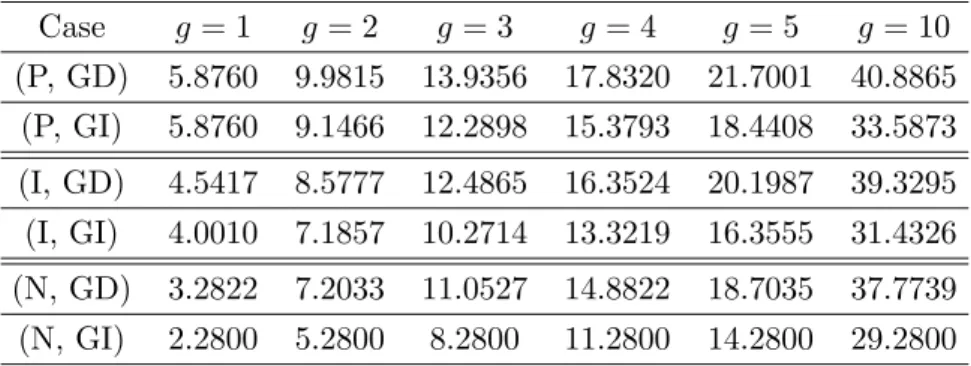
3.5.1 Impact of service time dependency . . . 63
3.5.2 Impact of variation of on- and off-periods . . . 64
3.5.3 Impact of correlation in on- and off-periods . . . 65
3.5.4 Impact of correlation between on-off and arrival processes . . . 68
4 Infinite-Server Queue 71 4.1 Introduction . . . 71
4.2 Model . . . 72
4.3 Time-Dependent Joint Distribution of the Number of Customers . . . 72
4.4 Numerically Feasible Formulas for Phase-Type Service Times . . . 75
4.4.1 Time-dependent joint binomial moments . . . 75
4.4.2 Time-dependent formula for phase-type services . . . 78
4.4.3 Limiting formula for phase-type services . . . 82
4.5 Numerical Examples . . . 84
4.5.1 Impact of service time distribution on Var[N] . . . 85
4.5.2 Impact of arrival process . . . 86
4.5.3 Impact of correlation in service time sequence . . . 89
5 Processor-Sharing Queue 93 5.1 Introduction . . . 93
5.2 Model and Known Results . . . 94
5.3 Sojourn Time Distribution . . . 94
5.4 Numerical Examples . . . 98
5.4.1 Numerical procedure and accuracy guarantee . . . 98
5.4.2 Impact of variation in inter-arrival times . . . 99
5.4.3 Impact of correlation in inter-arrival times . . . 99
5.5 Concluding Remarks . . . 101
CONTENTS xi
6 Conclusion 103
6.1 Summary of Results . . . 103 6.2 Future Work . . . 103
A Uniformization 105
B Queue Length Distribution in a BMAP/GI/1 Queue 107 C Total Queue Length Distribution in a FIFO Queue 111
D Proof of Lemma 3.2 115
E Proof of Theorem 3.5 117
F Total Queue Length Distribution in a Queue with Service Interruptions 119
G Proof of Lemma 4.1 121
List of Figures
1.1 The bivariate Markov process with the skip free to the right property. . . 13
1.2 The bivariate Markov process with the skip free to the left property. . . 16
2.1 Complementary distribution of total number of customers in Example 1. . . 44
2.2 Complementary distribution of total number of customers in Example 1. . . 45
2.3 Complementary distribution of total number of customers in Example 1. . . 45
3.1 Expected total queue length E[N]. . . 64
3.2 99.9 percentile (99.9 PT) of the total queue length. . . 66
3.3 Expected total queue length E[N]. . . 66
3.4 99.9 percentile (99.9 PT) of the total queue length. . . 67
3.5 Expected total queue length E[N]. . . 67
3.6 Conditional expected total queue length. . . 67
3.7 Conditional expected total queue length. . . 67
3.8 99.9 percentile (99.9 PT) of the total queue length. . . 69
3.9 Expected total queue length E[N]. . . 69
4.1 Limiting variance of the number of customers. . . 86
4.2 Limiting variance of the number of customers. . . 87
4.3 Time-dependent covariance Cov[N(t)] of the number of customers. . . 89
4.4 Time-dependent variance Var[N(t)] of the number of customers . . . 89
4.5 Variance and covariance in Case 1. . . 91
4.6 Variance and covariance in Case 2. . . 91
4.7 Variance and covariance in Case 3. . . 91
5.1 The computational domain of the hn,k. . . 99
5.2 The complementary distributionW(x) of the sojourn time. . . 100
5.3 The complementary distributionW(x) of the sojourn time. . . 100
xiii
List of Tables
2.1 Number of computedFm(n)’s in Example 1. . . 43
2.2 Number of stored ˘Fm(n)’s in Example 1. . . 44
2.3 Joint queue length distribution p(n1, n2)e. . . 46
2.4 Expected total number of customers in Example 1. . . 46
2.5 Expected total number of customers in Example 2. . . 47
3.1 Joint queue length distribution p(n1, n2)e. . . 65
xv
Chapter 1
Introduction
This chapter provides materials to be required in the following chapters and the brief survey of previous works on queues fed by multiple arrival streams with different service time distributions.
Throughout this thesis, we denote matrices and vectors by bold capital letters and bold small letters, respectively, and the empty sum is defined as zero.
1.1 Markovian Input Process
This section introduces an input process with batch Markovian arrival streams having different service time distributions. In this input process, customer arrivals from each arrival stream follow a BMAP [Luca91], which is an extension of a MAP [Luca90]. Therefore, after discussing MAP and BMAP [Luca91] in subsection 1.1.1, we formally define the input process with batch Markovian arrival streams in subsection 1.1.2.
1.1.1 Markovian arrival process
We begin with the definition of MAP. We consider a time homogeneous, stationary Markov chain with finite statesM={1, . . . , M}, which is assumed to be irreducible. The Markov chain is called the underlying Markov chain hereafter.
MAP is defined as follows. The underlying Markov chain stays in state i (i ∈ M) for an exponential interval of time with meanµ−1i . When the sojourn time in state i has elapsed, there are two possibilities: (1) With probability di,j, a transition to state j (j ∈ M) happens with an arrival. (2) With probabilityci,j (j∈ M,j6=i), a transition to statejhappens without an arrival.
Note that X
j∈M j6=i
ci,j+ X
j∈M
di,j = 1, for alli∈ M.
For the later use, we introduce two matrices, C and D. Let C denote an M ×M matrix whose (i, j)th (i, j∈ M) elementCi,j is given by
Ci,j =
( −µi, ifi=j, µici,j, otherwise.
1
LetD denote an M×M nonnegative matrix whose (i, j)th (i, j ∈ M) elementDi,j is given by Di,j =µidi,j.
Note that the infinitesimal generator of the underlying Markov chain is given byC+D. We define π as the stationary probability vector of the underlying Markov chain. Because of the finite state space M and the irreducibility of the underlying Markov chain, π is uniquely determined. Note thatπ satisfies
π(C+D) =0, πe= 1, (1.1)
where e denotes a column vector whose elements are all equal to one. The arrival rate λis then given by
λ=πDe.
We define N(t) and S(t) as the number of arrivals in time interval (0, t] and the state of the underlying Markov chain at time t, respectively. Further, let N(t, n) denote an M ×M matrix whose (i, j)th (i, j ∈ M) element represents
Pr [N(t) =n, S(t) =j|N(0) = 0, S(0) =i].
N(t, n)’s (t≥0, n= 0,1, . . .) satisfy the forward Chapman-Kolmogorov equations:
d
dtN(t, n) = N(t, n)C+N(t, n−1)D, t≥0, n= 1,2, . . . , N(0,0) = I,
whereI denotes an identity matrix with appropriate dimension. Thus, thez-transformN∗(t, z) of N(t, n) is given by
N∗(t, z) = exp [(C +zD)t].
As mentioned above, MAP can be characterized by (C,D).
In what follows, we show some special cases of MAP.
Example 1.1 Poisson process. ForC =−λand D =λ, MAP is reduced to a Poisson process with arrival rate λ.
Example 1.2 Phase-type (PH) renewal process. PH renewal process is defined in a very similar way to MAP except that the state of the underlying Markov chain immediately after an arrival is chosen according to a 1×M probability vector β, independent of its state immediately before the arrival. Namely,D = (−T e)β, where we use, by convention, T for C to distinguish PH renewal process from MAP. Note that theith (i∈ M) element ofM×1vector(−T e)represents the arrival (renewal) rate given the underlying Markov chain is in state i. Note also that inter-arrival (renewal) times are i.i.d. according to distribution function ψ(x):
ψ(x) = 1−βexp(Tx)e,
which is called the phase-type distribution with representation (β,T).
1.1. MARKOVIAN INPUT PROCESS 3 Example 1.3 Markov modulated Poisson process (MMPP).MMPP is a natural extension of a Poisson process, which has the arrival rate modulated by an M-state irreducible Markov chain.
To put it more concretely, the arrival rate takes M values λ1, . . . λM, and is equal to λj whenever the Markov chain is in state j. Let R denote the infinitesimal generator of the underlying Markov chain. Let Λ = diag(λ1, . . . λM). MMPP can then be characterized by R and Λ. Note here that this MMPP is equivalent to a MAP with representation (C,D), where
C =R−Λ, D=Λ.
We next discuss BMAP. The definition of BMAP is very similar to that of MAP except that multiple arrivals may happen simultaneously. Given the underlying Markov chain is in state i (i∈ M), it changes its state to state j (j ∈ M) at rate µidi,j(n) and narrivals occur at the same time. Besides, transitions with no arrivals are driven byC, as well as MAP. Note here thatdi,j(n)’s satisfy
X
j∈M j6=i
ci,j+ X
j∈M
X∞ n=1
di,j(n) = 1, for all i∈ M,
where ci,j denotes the (i, j)th element of C. Let D(n) denote an M ×M matrix whose (i, j)th (i, j∈ M) element Di,j(n) is given by
Di,j(n) =µidi,j(n).
Note that C +P∞n=1D(n) is the infinitesimal generator of the underlying Markov chain. Note further that the arrival rate λis given by
λ=π X∞ n=1
nD(n)e, (1.2)
whereπ denotes the stationary probability vector of the underlying Markov chain. Note also that N(t, n)’s for BMAP satisfy
d
dtN(t, n) = N(t, n)C+ Xn
m=1
N(t, n−m)D(m), t≥0, n= 1,2, . . . , N(0,0) = I.
It then follows from the above equations that the z-transform N∗(t, z) ofN(t, n) is given by N∗(t, z) = exp [(C +D∗(z))t],
where D∗(z) =
X∞ n=1
znD(n).
Thus, BMAP can be characterized by (C,D(n)).
1.1.2 Input process with batch Markovian arrival streams
It is assumed that there exist K (K ≥ 1) arrival streams. Customers arriving from the kth (k ∈ K = {1, . . . , K}) stream is called class k customers. Service times of class k customers are assumed to be i.i.d. according to a distribution functionHk(x) (x≥0) with finite mean hk.
As well as in subsection 1.1.1, we consider the underlying Markov chain with the finite state space M= {1, . . . , M} and assume its irreducibility. Customer arrivals happen in the following way. The underlying Markov chain stays in statei(i∈ M) for an exponential interval of time with meanµ−1i , and then changes its state to statej(j ∈ M) with probabilityσi,j, wherePj∈Mσi,j = 1 for alli(i∈ M). When a transition from stateito state j happens,nk (k∈ K) classkcustomers simultaneously arrive at the queue with probability σi,j(n1, . . . , nK)/σi,j, where σi,i(0, . . . ,0) is assumed to be zero for alli(i∈ M), andσi,j(n1, . . . , nK) satisfies
σi,j = X∞ n1=1
· · · X∞ nK=1
σi,j(n1, . . . , nK).
The assumptionσi,i(0, . . . ,0) = 0 (∀i∈ M) implies that at least one customer arrives whenever a transition from any stateito itself happens.
We now introduce some notations to describe the above input process. We define C as an M×M matrix whose (i, j)th elementCi,j is given by
Ci,j =
( −µi, i=j, σi,j(0)µi, otherwise,
where0 denotes a vector of zeros with appropriate dimension. We also defineZ and Z+ as Z = {(n1, . . . , nK); nk= 0,1, . . . for all k∈ K},
Z+ = Z − {0},
respectively. Letndenote a 1×Knonnegative vector (n1, . . . , nK). We then defineD(n) (n∈ Z+) as an M×M matrix whose (i, j)th elementDi,j(n) is given by
Di,j(n) =σi,j(n)µi, n∈ Z+.
When a state transition driven byD(n) occurs,nkcustomers of each classksimultaneously arrive.
On the other hand, when a state transition driven by C occurs, no customers arrive. Note here that the infinitesimal generator of the underlying Markov chain is given by C +D, where D is defined as
D = X
n∈Z+
D(n). (1.3)
Thus, the counting process of arrivals is characterized by (C,D(n)).
Example 1.4 Suppose that
D(n) =O if n∈ Z − {e1,e2, . . . ,eK},
1.2. MARKOV CHAINS SKIP FREE TO ONE DIRECTION 5 where O denotes a matrix of zeros and ek denotes the kth unit vector:
ek = (
z }|K { 0, . . . ,0,1,0, . . . ,0 ).
kth
(1.4) This assumption means that at most one arrival from an arrival stream happens at any time. This special case is called marked MAP (MMAP) in [He96].
Finally, we consider the marginal arrival process of the kth (k∈ K) stream. We defineCek and fDk(n) (n= 1,2, . . .) as
Cek=C+ X
n∈Z+ nk=0
Dk(n), fDk(n) = X
n∈Z+ nk=n
Dk(n),
respectively. Note thatCek andDfk(n) satisfy Cek+
X∞ n=1
Dfk(n) =C+D.
When a transition driven byDfk(n) happens,ncustomers of classkarrive at the queue. Besides, a transition driven byCek happens without a class kcustomer. Thus, the marginal arrival process of thekth stream is a BMAP with representation (Cek,Dfk(n)). We define λk (k∈ K) as the arrival rate of classk customers, i.e.,
λk=π X∞ n=1
nfDk(n)e,
where π denotes the invariant probability vector for C+D. Let ρk denote the utilization factor of class k customers, i.e., ρk = λkhk. Note that the overall arrival rate λand utilization factor ρ are given by
λ= X
k∈K
λk, ρ= X
k∈K
ρk,
respectively. Note also that in a work-conserving single-server queue,ρ <1 ensures that the system is stable [Loyn62].
1.2 Markov Chains Skip Free to One Direction
This section summarizes analytical results on time-homogeneous Markov chains with the skip free to one direction and spatial homogeneity properties. Markov chains with these properties are classified into two cases, i.e., the skip free to the left case and to the right case, which are natural extensions of embedded Markov chains in an M/G/1 queue and GI/M/1 queue, respectively. Such Markov chains now play a vital role in algorithmic analysis of the queue length distribution. In what follows, we first introduce Markov chains with the skip free to the right/left properties and briefly discuss the steady-state solutions of these two types of Markov chains in subsections 1.2.1 and 1.2.2.
In a single-server queue, let Xk− and Dk denote the number of customers immediately before the kth arrival and the number of departures during the kth inter-arrival time, respectively. We then have
Xk+1− = max(Xk−+ 1−Dk+1,0), k= 0,1, . . . .
We now consider a GI/M/1 queue, where inter-arrival times are i.i.d. according to a distribution functionG(x) with mean λ−1 and service times are exponential with meanµ−1. In such a queue, Dk’s are i.i.d. random variables, and hence the sequence{Xk−;k= 0,1, . . .} of random variables is a Markov chain with transition probability matrix:
f0 e0 0 0 · · · f1 e1 e0 0 · · · f2 e2 e1 e0 · · · f3 e3 e2 e1 · · · f4 e4 e3 e2 · · · ... ... ... ... . ..
,
where en=
Z ∞
0
e−µx(µx)n
n! dG(x), fn= X∞ m=n+1
em.
If ρ =λ/µ < 1, the Markov chain {Xk−;k = 0,1, . . .} has the stationary distribution. Assuming ρ <1, we define qGI/M/1(n) (n= 0,1, . . .) as limk→∞Pr[Xk−=n]. ThenqGI/M/1(n) is given by
qGI/M/1(n) =γn(1−γ), n= 0,1, . . . , (1.5)
whereγ is a positive number satisfying γ =P∞n=0enγn and γ <1. The assumption ρ <1 ensures thatγ is uniquely determined.
On the other hand, in a single-server queue, let Xk+ and Ak denote the number of customers immediately after the kth departure and the number of arrivals during thekth service time. We then have
Xk+1+ = max(Xk+−1,0) +Ak+1.
We consider an M/G/1 queue, where arrivals follow Poisson process with a rate λ and service times are i.i.d. according to a distribution H(x) with mean µ−1. In the M/G/1 queue, Ak’s are i.i.d. random variables, and hence{Xk+;k= 0,1, . . .}is a Markov chain with transition probability matrix:
a0 a1 a2 a3 · · · a0 a1 a2 a3 · · · 0 a0 a1 a2 · · · 0 0 a0 a1 · · · 0 0 0 a0 · · · ... ... ... ... . ..
,
1.2. MARKOV CHAINS SKIP FREE TO ONE DIRECTION 7 where
an= Z ∞
0
e−λx(λx)n
n! dH(x).
If ρ = λ/µ < 1, the Markov chain {Xk+;k = 0,1, . . .} has the stationary distribution. Under the assumption ρ < 1, we define qM/G/1(n) (n = 0,1, . . .) as limk→∞Pr[Xk+ =n]. Then qM/G/1(n)’s are recursively determined in the following way.
qM/G/1(0) = 1−ρ, qM/G/1(n) =
"
qM/G/1(0)an+
n−1X
m=1
qM/G/1(m)an+1−m
#
(1−a1)−1, n= 1,2, . . . , where
an= X∞ m=n
am.
Note that Markov chains {Xk−;k = 0,1, . . .} and {Xk+;k = 0,1, . . .} have the following two properties. One is the spatial homogeneity except for the boundary part (e.g., if Xk+ ≥ 1, Xk+ increases by n−1 with probability an). The other is the skip free to one direction property. To put it more concretely, the Markov chain{Xk−;k= 0,1, . . .}(resp.{Xk+;k= 0,1, . . .}) can increase (resp. decrease) at most by one when a transition happens. This is called theskip free to the right (resp. left) property.
Next we consider a GI/PH/1 queue and a PH/G/1 queue, where the service time distribu- tion and the inter-arrival time distribution are of phase-type with representation (βH,TH) and (βA,TA), respectively. Let G(x) and H(x) denote the inter-arrival distribution in the GI/PH/1 queue and the service time distribution in the PH/G/1 queue, respectively. Note that Dk’s in the GI/PH/1 queue and Ak’s in the PH/G/1 queue are non-i.i.d. random variables. However, Dk+1 (resp. Ak+1) is conditionally independent of the past history {Dl;l = 1, . . . , k} (resp. {Al;l = 1, . . . , k}), given the state Jk− (resp.Jk+) of the phase-type distribution (βH,TH) (resp. (βA,TA)) immediately before (resp. after) the kth arrival (resp. departure). Thus,{(Xk−, Jk−);k = 0,1, . . .} is a bivariate Markov chain whose transition probability matrix is given by
PGI/PH/1 =
F0 E0 O O · · · F1 E1 E0 O · · · F2 E2 E1 E0 · · · F3 E3 E2 E1 · · · F4 E4 E3 E2 · · · ... ... ... ... . ..
, (1.6)
whereEn’s (n= 0,1, . . .) satisfy X∞
n=0
znEn= Z ∞
0
exp [(TH +z(−THe)βH)x]dG(x),
and Fn=
X∞ m=n+1
EmeβH, n= 0,1, . . . .
Similarly,{(Xk+, Jk+);k= 0,1, . . .} is a bivariate Markov chain whose transition probability matrix is given by
PPH/G/1 =
B0 B1 B2 B3 · · · A0 A1 A2 A3 · · · O A0 A1 A2 · · · O O A0 A1 · · · O O O A0 · · · ... ... ... ... . ..
, (1.7)
whereAn’s (n= 0,1, . . .) satisfy X∞
n=0
znAn= Z ∞
0 exp [(TA+z(−TAe)βA)x]dH(x), and
Bn=eβAAn, n= 0,1, . . . .
We can see from (1.6) and (1.7) that these two bivariate Markov chains have the spatial homo- geneity (except for the boundary part) and the skip free to one direction property with respect to the first variables, i.e.,Xk− and Xk+. As mentioned above, the queue length processes in queues we often encounter are reduced to bivariate Markov chains with these two properties. In general, if a bivariate Markov chain has a transition probability matrix with the same structure as
PR=
F0 Eb0 O O · · · F1 E1 E0 O · · · F2 E2 E1 E0 · · · F3 E3 E2 E1 · · · F4 E4 E3 E2 · · · ... ... ... ... . ..
, (1.8)
it is called a Markov chain of G/M/1 type. Further, a bivariate Markov chain has a transition probability matrix with the same structure as
PL=
B0 B1 B2 B3 · · · Ab0 A1 A2 A3 · · · O A0 A1 A2 · · · O O A0 A1 · · · O O O A0 · · · ... ... ... ... . ..
, (1.9)
1.2. MARKOV CHAINS SKIP FREE TO ONE DIRECTION 9 it is called a Markov chain of M/G/1 type. These two Markov chains can be considered as extensions of the Markov chains describing the queue length processes in the GI/M/1 queue and the M/G/1 queue, respectively, in the sense that each element of a transition probability matrix is replaced by a block matrix. This is the origin of their names.
Remark 1.1 Some researchers have studied G/M/1-type and M/G/1-type Markov chains with a tree structure. For G/M/1-type Markov chains with a tree structure, matrix product-form solutions are obtained by Yeung and Sengupta [Yeun94]. As for M/G/1-type Markov chains with a tree structure, He [He00a, He00b, He03a] studied conditions for them to be positive recurrent, null recurrent or transient. A related work is found in [He03b], which studied sufficient conditions for stability or instability of a single-server queue with LCFS preemptive-repeat service discipline.
Further, Takine et al. [Taki95] established a paradigm to compute the steady-state solution of the M/G/1-type Markov chain with a tree structure under the assumption that it is irreducible and positive recurrent. That paradigm is an extension of the M/G/1 paradigm [Neut89].
1.2.1 Markov chains of G/M/1 type
In this subsection, we consider a G/M/1-type Markov chain {(Xk−, Jk−);k= 0,1, . . .}with a tran- sition probability matrix PR in (1.8), where En, Fn (n = 0,1, . . .) and Eb0 denotes M1−×M1−, Mmin(n,1)− ×M0− and M0−×M1− matrices, respectively.
We define E as E =
X∞ n=0
En.
Note here thatE is a stochastic matrix.
We now assume the following:
Assumption 1.1 E is irreducible.
We then defineνE as a 1×M1− vector satisfying νEE=νE, νEe= 1.
Note that Assumption 1.1 ensures that νE is uniquely determined. We also make the following assumption:
Assumption 1.2
(a) The G/M/1-type Markov chain {(Xk−, Jk−);k= 0,1, . . .} is irreducible, and (b) νE
X∞ n=1
nEne>1.
Remark 1.2 The irreducible G/M/1-type Markov chain{(Xk−, Jk−);k= 0,1, . . .} is positive recur- rent if and only if Assumption 1.4 (b) holds (See Corollary 3.3 on page 319 in [Asmu03]).
We define X− and J− as generic random variables for Xk− and Jk−, respectively, in steady sate. Let x− = (x−0,x−1, . . .) denote the steady-sate solution for the G/M/1-type Markov chain {(Xk−, Jk−);k = 0,1, . . .}, wherex−n denotes a 1×Mmin(n,1)− vector whose jth element represents Pr[X− =n, J−=j]. Let Rdenote the minimal nonnegative solution [Neut81] of
R= X∞ n=0
RnEn.
R is called a rate matrix and has the following probabilistic meanings [Neut81]. We consider a cycle of visits to the state set {(n, ν);ν = 1, . . . , M1−} (n ≥ 1). The (i, j)th element of R then represents the mean number of visits on state (n+ 1, j) during a cycle that starts with state (n, i).
In terms of rate matrixR,x− = (x−0,x−1, . . .) is given in the following way.
Proposition 1.1 ([Neut81]) x−0 and x−1 are determined by x−0 = x−0F0+x−1
X∞ m=1
Rm−1Fm,
x−1 = x−0Eb0+x−1 X∞ m=1
Rm−1Em, x−0e + x−1(I−R)−1e= 1,
and for n= 2,3, . . .,
x−n =x−1Rn−1. (1.10)
Thex−n can be considered as a matrix version of the geometric solution (1.5) for the GI/M/1 queue, and it is called thematrix geometricsolution.
1.2.2 Markov chains of M/G/1 type
In this subsection, we consider an M/G/1-type Markov chain {(Xk+, Jk+);k = 0,1, . . .} with a transition probability matrixPL in (1.9), whereAn,Bn(n= 0,1, . . .) andAb0 denotesM1+×M1+, M0+×Mmin(n,1)+ and M1+×M0+ matrices, respectively. We defineµA andµB as
µA= X∞ n=1
nAne, µB= X∞ n=1
nBne,
respectively. We also defineA and B as A=
X∞ n=0
An, B= X∞ n=1
Bn,
respectively. Note thatA is a stochastic matrix andB0e+Be=e.
We now assume the following:
Assumption 1.3 A is irreducible.
1.2. MARKOV CHAINS SKIP FREE TO ONE DIRECTION 11 LetνA denote a 1×M1+ vector satisfying
νAA=νA, νAe= 1.
Note that Assumption 1.3 ensures that νA is uniquely determined. We defineρAas ρA=νAµA.
In what follows, we also make the following assumption:
Assumption 1.4
(a) The M/G/1-type Markov chain {(Xk+, Jk+);k= 0,1, . . .} is irreducible, (b) µB is a finite vector, and
(c) ρA<1.
Remark 1.3 The irreducible M/G/1-type Markov chain{(Xk+, Jk+);k= 0,1, . . .} is positive recur- rent if and only if Assumption 1.4 (b) and (c) hold (See Proposition 3.1 on page 318 in [Asmu03]).
We define X+ and J+ as generic random variables for Xk+ and Jk+, respectively, in steady state. Let x+ = (x+0,x+1, . . .) denote the steady-state solution for the M/G/1-type Markov chain {(Xk+, Jk+);k = 0,1, . . .}, where x+n denotes a 1×Mmin(n,1)+ vector whose jth element rep- resents Pr[X+ = n, J+ = j]. The numerical algorithm to compute the steady-state solution x+= (x+0,x+1, . . .) is called the M/G/1 paradigm, where anM1+×M1+ matrixGplays a vital role [Neut89]. The (i, j)th element ofGrepresents the probability that forn≥2, the first passage time from state (n, i) to any state in {(n−1,1), . . . ,(n−1, M1+)} ends with state (n−1, j). The Gis often called the fundamental matrix. It is known that Gis the minimal nonnegative solution of [Neut89]
G= X∞ n=0
AnGn.
The computation ofGis referred to [Neut89, Luca91]. In terms ofG, we defineM0+×M0+ matrix K as
K =B0+ X∞ m=1
BmGm−1
"
I− X∞ l=1
AlGl−1
#−1
Ab0. (1.11)
Further, letκ denote a 1×M0+ vector satisfying κK =κ, κe= 1.
We now show a recursive formula for the computation ofx+n’s (n= 0,1, . . .).
Proposition 1.2 ([Rama88, Sche90]) x+0 is given by x+0 =
"
1 + κ
1−ρA
(
µB+ B− X∞ l=1
BlGl
!
[I −A+eνA]−1µA )#−1
κ,
andx+n’s (n= 1,2, . . .) are recursively determined by x+n =
"
x+0Bn+
n−1X
l=1
x+l An−l+1
#
[I−A1]−1, where
Bν = X∞ m=0
Bm+νGm, Aν = X∞ m=0
Am+νGm.
1.3 Markov Processes Skip Free to One Direction
This section considers time-homogeneous Markov processes with the skip free to one direction and spatial homogeneity properties, which are continuous analogs of Markov chains discussed in section 1.2. These Markov processes are also classified into two cases, i.e., the skip free to the left case and to the right case, and they are very important models to analyze the waiting time distribution and the virtual waiting time distribution in single-server queues.
1.3.1 Markov processes skip free to the right
This subsection considers a bivariate Markov process{(XR(t), JR(t));t≥0} with the skip free to the right property. We formally define it as follows:
(a) XR(t) takes values on [0,∞) and JR(t) takes integer values on M = {1, . . . , M}. Further, XR(t) is skip free to the right and increases at a liner rate of one if there are no downward jumps.
(b) Given (XR(t), JR(t)) = (x, i) (x > 0, i ∈ M), the bivariate Markov process can change its state to somewhere between (x −y, j) and (x−y+dy, j) (0 ≤ y < x, j ∈ M) at a rate dEi,j(y). Let E(y) denote an M ×M matrix whose (i, j)th element is given byEi,j(y). To avoid trivialities, Ei,i(0) = 0 (∀i ∈ M) is assumed. Further, E(∞) is assumed to be an irreducible matrix.
(c) Given (XR(t), JR(t)) = (x, i) (x > 0, i ∈ M), the bivariate Markov process can change its state to state (0, j) (j ∈ M) at rate Fjump,i,j(x). Let Fjump(x) denote an M ×M matrix whose (i, j)th element is given byFjump,i,j(x). It is assumed that Fjump(∞) =O.
We define Ejump(x) (x≥0) and Ejump(∞) as Ejump(x) = E(x)−E(0),
Ejump = E(∞)−E(0),
1.3. MARKOV PROCESSES SKIP FREE TO ONE DIRECTION 13 respectively. Note that these two matrices are nonnegative. We also define Eslope as an M ×M matrix whose (i, j)th element Eslope,i,j is given by
Eslope,i,j =
Ei,j(0), ifi6=j,
− X
ν∈M
Ei,ν(∞), otherwise.
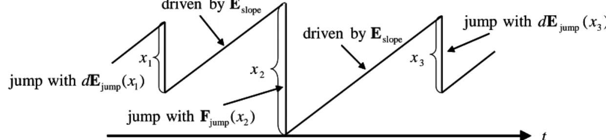
Note that Eslope +Ejump is the infinitesimal generator of an irreducible Markov chain. Thus, {(XR(t), JR(t));t≥0} can be characterized by Eslope,Ejump(x) andFjump(x) as shown in Figure 1.1
) ( with
jump dEjump x1
) ( with
jump dEjump x3
slope
by driven E
slope
by driven E
x2 x3
t )
( with
jump Fjump x2 x1
) ( with
jump dEjump x1
) ( with
jump dEjump x3
slope
by driven E
slope
by driven E
x2 x3
t )
( with
jump Fjump x2 x1
Figure 1.1: The bivariate Markov process with the skip free to the right property.
Proposition 1.3 [Seng89]A necessary and sufficient condition for the irreducible Markov process {(XR(t), JR(t));t≥0} to be positive recurrent is
ηE Z ∞
0 xdEjump(x)e>1,
where ηE denotes the 1×M invariant probability vector for Eslope+Ejump.
In the rest of this subsection, we assume that {(XR(t), JR(t));t ≥ 0} is positive recurrent and discuss the steady-state density of{(XR(t), JR(t));t≥0}.
LetπR(x) denote a 1×M vector whosejth element πR,j(x) represents πR,j(x)dx= lim
t→∞
1 t
Z t
0 1{x≤XR(τ)≤x+dx, JR(τ) =j}dτ,
where 1{χ} denotes an indicator function of eventχ Then, standard flow conservation arguments yield
πR(x) =πR(x−∆x)(I +Eslope∆x) + Z ∞
0
πR(x+u)dEjump(u)∆x+o(∆x), x >0,(1.12) and
πR(0) = Z ∞
0
πR(u)dFjump(u).
Rearranging terms in (1.12), dividing both sides by ∆xand taking their limits as ∆x→0, we have d
dxπR(x) =πR(x)Eslope+ Z ∞
0
πR(x+u)dEjump(u), x >0.
Further, from the total probability law, we have Z ∞
0
πR(x)edx= 1.
We now introduce an M ×M irreducible matrix Θ, which characterizes πR(x) (x ≥ 0). We consider the sequence of matrices {Θn;n= 0,1, . . .} withΘ0 =Eslope and
Θn=Eslope+ Z ∞
0 exp(Θn−1x)dEjump(x), n= 1,2, . . . .
It is known [Seng89] that if {(XR(t), JR(t));t ≥ 0} is positive recurrent, Θ = limn→∞Θn exists and the limit matrixΘis the minimal solution of
Θ=Eslope+ Z ∞
0
exp(Θx)dEjump(x).
Note here that Θ is non-singular and has strictly negative diagonal elements and nonnegative off-diagonal elements [Seng89].
Proposition 1.4 [Seng89] The steady-state density πR(x) (x≥0) is given by πR(x) =πR(0) exp(Θx), x >0,
where πR(0) satisfies πR(0) =πR(0)
Z ∞
0
exp(Θx)Fjump(x)dx, πR(0)(−Θ)−1e= 1.
We close this subsection by showing an important application of the above result.
We consider the waiting time distribution in a stationary FIFO GI/PH/1 queue. Service times are assumed to be i.i.d. according to a phase-type distribution with representation (β,T), whereβ denotes a 1×M probability vector andT denotes an M ×M irreducible and defective generator.
We define τ as τ = −T e. Let G(x) denote the inter-arrival time distribution. We assume that G(0+) = 0. For the stationary GI/PH/1 queue, we define a bivariate process{(W(t), S(t));t≥0}, where W(t) and S(t) denotes the attained waiting time and the phase of service, respectively, at time t. If no customers are present in the system at time t, W(t) and S(t) are set to zero. Note that the {W(t);t ≥ 0} increases at a rate of one as long as a customer is in service and jumps downward when a customer in the server departs from the system. The amount of the downward jump is equal to the inter-arrival time between the departing customer and the customer served next to him, unless the departure corresponds to the end of a busy period. Otherwise,W(t) jumps to zero.
We now construct another process by deleting all times when W(t) and J(t) are equal to zero and gluing together all non-zero realizations of {(W(t), S(t));t ≥ 0}. It is easy to see that the resulting process is equivalent to{(XR(t), JR(t));t≥0}with
Eslope = T,
Ejump(x) = τ βG(x), (1.13)
Fjump(x) = τ β(1−G(x)), (1.14)
1.3. MARKOV PROCESSES SKIP FREE TO ONE DIRECTION 15 where Te denote a diagonal matrix whose jth diagonal element is given by the (j, j)th element of T. Thus, from Proposition 1.4, the steady-state densityπR(x) (x >0) is given by
πR(x) =−αΘexp(Θx), x >0, (1.15)
whereα is a invariant probability vector for (T +τ β) and Θsatisfies Θ=T +
Z ∞
0
exp(Θx)dG(x)τ β. (1.16)
Let tk denote the time when the kth downward jump happens, i.e., the kth customer departs from the system. Note that the waiting time of (k+ 1)th customer is equivalent to XR(tk+). It is clear from (1.13) and (1.14) thatXR(tk+) and JR(tk+) are independent. Thus, the waiting time distributionWq(x) is given by
Wq(x) = Z ∞
0
Z x+u
0
πR(y)τ ατ dy
dG(u), (1.17)
Substituting (1.15) and (1.16) into (1.17), we obtain Wq(x) = 1− 1
µexp(Θx)(Θ−T)e,
whereµ=ατ is the reciprocal of the mean service time.
1.3.2 Markov processes skip free to the left
In this subsection, we consider a bivariate Markov process{(XL(t), JL(t));t≥0}with the skip free to the left property, which is formally defined as follows:
(a) XL(t) takes values on [0,∞) and JL(t) takes integer values on M = {1, . . . , M}. Further, XL(t) is skip free to the left and decreases at a liner rate of one if there are no upward jumps.
(b) Given (XL(t), JL(t)) = (x, i) (x > 0, i ∈ M), the bivariate Markov process can change its state to somewhere between (x+y, j) and (x+y+dy, j) (y≥0, j ∈ M) at a ratedAi,j(y). Let A(y) denote anM×M matrix whose (i, j)th element is given byAi,j(y). To avoid trivialities, Ai,i(0) = 0 (∀i∈ M) is assumed. Further,A(∞) is assumed to be an irreducible matrix.
(c) Given (XL(t), JL(t)) = (0, i) (i ∈ M), the bivariate Markov process can change its state to somewhere between (y, j) and (y+dy, j) (y ≥0, j ∈ M) with probability dBjump,i,j(y). Let Bjump(y) denote an M ×M matrix whose (i, j)th element is given by Bjump,i,j(y), where Bjump(∞) is assumed to be a stochastic matrix. This means that an upward jump happens with probability one whenXL(t) = 0.
For later use, we introduce some matrices. We define Ajump(x) (x≥0) and Ajump as Ajump(x) = A(x)−A(0),
Ajump = A(∞)−A(0),
respectively. Note that these two matrices are nonnegative. We also defineAslope as an M ×M matrix whose (i, j)th element Aslope,i,j is given by
Aslope,i,j =
Ai,j(0), ifi6=j,
− X
ν∈M
Ai,ν(∞), otherwise.
Note that Aslope has strictly negative diagonal elements and nonnegative off-diagonal elements.
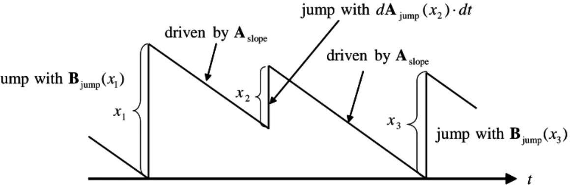
Note also that Aslope +Ajump is an irreducible generator of a Markov chain and hence has the invariant probability vector ηA. Thus, {(XL(t), JL(t));t ≥ 0} can be characterized by Aslope, Ajump(x) and Bjump(x), as shown in Figure 1.2.
) ( with
jump Bjump x1
dt x
d ( )⋅
with
jump Ajump 2
slope
by driven A
slope
by driven A
x1
x2
x3
t ) ( with
jump Bjump x3 )
( with
jump Bjump x1
dt x
d ( )⋅
with
jump Ajump 2
slope
by driven A
slope
by driven A
x1
x2
x3
t ) ( with
jump Bjump x3
Figure 1.2: The bivariate Markov process with the skip free to the left property.
In what follows, we discuss the steady-state behavior of {(XL(t), JL(t));t ≥0}. To do so, we first show a necessary and sufficient condition for its positive recurrence.
Proposition 1.5 [Taki96]A necessary and sufficient condition for the irreducible Markov process {(XL(t), JL(t));t≥0} to be positive recurrent is
ηAajump<1, and
Z ∞
0
xdBjump(x)
i
<∞ (i∈ M), where
ajump= Z ∞
0
xdAjump(x)e.
Hereafter, we assume that{(XL(t), JL(t));t≥0} is positive recurrent. LetπL(x) denote a 1×M vector whosejth elementπL,j(x) represents
πL,j(x)dx= lim
t→∞
1 t
Z t
0 1{x≤XL(τ)≤x+dx, JL(τ) =j}dτ.
We defineΠL(x) as ΠL(x) =
Z x
0
πL(y)dy.
![Figure 3.1 plots the expected total queue lengths E[N ] in Cases GD and GI as functions of α −1](https://thumb-ap.123doks.com/thumbv2/123deta/7309029.2421397/81.892.100.777.242.355/figure-plots-expected-total-queue-lengths-cases-functions.webp)
![Figure 3.1: Expected total queue length E[N ].](https://thumb-ap.123doks.com/thumbv2/123deta/7309029.2421397/82.892.224.566.194.510/figure-expected-total-queue-length-e-n.webp)
![Figure 3.3: Expected total queue length E[N ].](https://thumb-ap.123doks.com/thumbv2/123deta/7309029.2421397/84.892.478.774.125.394/figure-expected-total-queue-length-e-n.webp)
![Figure 3.5: Expected total queue length E[N ].](https://thumb-ap.123doks.com/thumbv2/123deta/7309029.2421397/85.892.94.422.179.474/figure-expected-total-queue-length-e-n.webp)
