Keywords |Active learning, Multilayer perceptron, Fisher information matrix, Pruning.

Statistical Active Learning in Multilayer

Perceptrons

Kenji Fukumizu

Brain Science Institute, RIKEN Hirosawa 2-1, Wako Saitama 351-0198 Japan

Tel: +81-48-467-9664 Fax: +81-48-467-9693 E-mail: [email protected]

Abstract |This paper proposes new methods of generating input locations actively in gathering training data, aiming at solving problems special to multilayer perceptrons. One of the problems is that the optimum input locations which are calculated deterministically sometimes result in badly- distributed data and cause local minima in back-propagation training. Two probabilistic active learning methods, which utilize the statistical variance of locations, are proposed to solve this problem. One is parametric active learning and the other is multi-point-search active learning. Another se- rious problem in applying active learning to multilayer per- ceptrons is the singularity of a Fisher information matrix, whose regularity is assumed in many methods including the proposed ones. A technique of pruning redundant hidden units is proposed to keep the regularity of a Fisher infor- mation matrix, which makes active learning applicable to multilayer perceptrons. The eectiveness of the proposed methods is demonstrated through computer simulations on simple articial problems and a real-world problem in color conversion.

Keywords |Active learning, Multilayer perceptron, Fisher information matrix, Pruning.

I. Introduction

W

HEN we train a learning machine like a feedforward neural network to estimate the true input-output re- lation of the target system, we must prepare input vectors, observe the corresponding output vectors, and pair them to make training data. It is well known that we can im- prove the ability of a learning machine by designing the input of training data. Such methods of selecting the loca- tion of input vectors have been long studied in the name of experimental design ([1]), response surface methodology ([2]), active learning ([3],[4]), and query construction ([5]).

They are especially important when collecting data is very expensive.

This paper discusses statistical active learning methods for the multilayer perceptron (MLP) model. We consider learning of a network as statistical estimation of a regres- sion function. The accuracy of the estimation is often eval- uated using the generalization error, which is the mean square error between the true function and its estimate. In this paper, the objective of active learning is to reduce the generalization error. Using the statistical asymptotic the- K. Fukumizu is with the Brain Science Institute, RIKEN, Saitama, Japan. E-mail: [email protected]

ory, we can derive a criterion on where are eective input locations to minimize the generalization error ([6]).

The main purpose of this paper is to solve prob- lems related to special properties of multilayer networks.

One problem is that a learning rule like the error back- propagation cannot always achieve the global minimum of the training error, while many statistical active learning or experimental design methods assume its availability. We see that learning with the optimal data which are calcu- lated deterministically is trapped by local minima more often than passive learning. To overcome this problem, we propose probabilistic methods, which generate an input data with deviation from the optimal location.

Another problem is caused by the singularity of a Fisher information matrix. Many statistical active learning meth- ods assume the regularity of a Fisher information ma- trix ([1],[4],[6]), which plays an important role in the asymptotic behavior of the least square error estimator ([7],[8],[9],[10],[11]). The Fisher information matrix of a MLP, however, can be singular if the network has redun- dant hidden units. Since active learning methods usually require that the prepared model includes the true function, the number of hidden units must be large enough to realize it with high accuracy. Thus, the model tends to be redun- dant especially in active learning. To solve this problem, we propose active learning with hidden unit pruning based on the regularity condition of a Fisher information matrix of a MLP ([12]). The method removes redundant hidden units to keep the regularity of a Fisher information matrix, and makes active learning methods applicable to the MLP model.

This paper is organized as follows. In Section II, we give

basic denitions and terminology, and describe an active

learning criterion. In Section III, we propose two novel ac-

tive learning methods based on the probabilistic optimality

of training data. In Section IV, we explain a problem con-

cerning the singularity of a Fisher information matrix, and

propose a pruning technique. Section V demonstrates the

eectiveness of the proposed methods through an applica-

tion to a real-world problem, and Section VI concludes this

paper.

II. Active learning in statistical learning A. Basic denitions and terminology

First, we give basic denitions and terminology, which our active learning methods are based on.

We discuss the three-layer perceptron model dened by

f

i

( x ^{; ) = X}

j

=

w

ij s

X

k

=

u

jk x

k

+

!

+

(

) (1) where ^{= (}

¹¹

¹

¹¹

1

) represents weights and biases, and

(

) = ₁₊ ¹

is the sigmoidal function.

We assume that the target system which is estimated by a network is a function f ⁽ x ), and the output of the system is observed with an additive Gaussian noise. Then, an output data y ^follows

y ⁼ f ⁽ x ^{) +} Z

⁽²⁾

where Z is a random vector with a zero mean and a scalar covariance

²

. To obtain a set of training data

=

f

( x ⁽

⁾

y ⁽

^{) )}

⁼

, we prepare input vectors

X

N

=

x ⁽

⁾

, feed them to the target system, and observe output vectors

y ⁽

⁾

subject to eq.(2). The problem of active learning is how to prepare

.

When a set of training data

is given, we employ the least square error (LSE) estimator ^ ^{, that is,}

^ ^{= argmin}

X

=1

k

y ⁽

⁾

f ⁽ x ⁽

^{) ; )}

⁽³⁾

Unlike linear models whose experimental design has been extensively studied in the eld of statistics ([1]), the solu- tion of eq.(3) cannot be rigorously calculated in the case of neural networks. An iterative learning rule like the er- ror back-propagation is needed to obtain an approximation of ^ . To derive an active learning criterion, however, we assume the availability of ^ . A problem related to this assumption is discussed later.

We use the generalization error to evaluate the ability of a trained network. For the denition, we introduce the environmental probability

, which gives independent input vectors in the actual environment where a trained network should be located. In system identication, for example,

represents the distribution of input vectors which are given to the system. The generalization error is dened by

E

gen

= ^Z

f ⁽ x ^{; ^ )}

f ⁽ x ⁾

⁽ x ⁾

⁽⁴⁾

which is the mean square error between the true function and its estimate. The purpose of our active learning meth- ods is to reduce the expectation of the generalization er- ror E[

]. The expectation E[

] is taken with respect to training data, as ^ is a random vector depending on the statistical training data

.

If the input vectors

x ⁽

⁾

are independent samples from the environmental distribution

, such learning is called passive. Active learning is, of course, expected to be supe- rior to passive learning with respect to the generalization error. When the number of training data is suciently large, and if the true function is included in the model, the statistical asymptotic theory tells that E[

] of passive learning is approximately

, where

is the dimension of ([8],[10]).

B. Criterion of statistical active learning

Because our principle of learning is to minimize the ex- pectation of the generalization error, in order to construct an active learning method we must evaluate how E[

] depends on

. There are several kinds of methods, in general, to estimate the generalization error. One is to use the statistical asymptotic theory ([7]), and another one is to use resampling techniques like bootstrap ([13]) or cross- validation ([14]). The concept of structural risk minimiza- tion (SRM, [15]) developed by Vapnik also gives a solid basis to discuss generalization problems. In this paper, we employ a method based on the asymptotic theory. The resampling techniques, which estimate the generalization error using given training data, is not suitable for active learning in which we have to know how the generalization error depends on an input point before the data is actually generated. We do not adopt the SRM principle either, be- cause it is based on the bound of the worst case unlike our objective to minimize the expectation of the generalization error.

For the approximation of eq.(4), we assume that the true function f ⁽ x ) is completely included in the model and

f ⁽ x ^;

^{) =} f ⁽ x ). This assumption is not rigorously satis- ed in practical problems. In general, the expectation of the generalization error can be decomposed as

E[

] = E ^Z

f ⁽ x ^{; ^ )}

f ⁽ x ^;

⁾

⁽ x ⁾

+ ^Z

f ⁽ x ^;

⁾

f ⁽ x ⁾

⁽ x ⁾

⁽⁵⁾

where

is the parameter that gives min

^R

f ⁽ x ^;

⁾

f ⁽ x ⁾

⁽ x ). The rst and the second terms in eq.(5) are called the variance and the bias of the model respectively.

Moody ([16]), for example, discusses the generalization er- ror in the framework of nonparametric regression which allows the model bias. However, it is very dicult to de- scribe explicitly the dependence of E[

] on

if the model bias exists. Therefore, we assume that the bias of the model is small enough to be neglected, and that active learning is supposed to reduce the variance term. In Sec- tion IV, we discuss how to solve the problem of the model bias.

Similar to Cohn's discussion ([4]), application of the asymptotic theory ([9],[10]) or local linearization under the bias-free assumption shows

E[

]

² Tr

(

⁾

^{1 (}

^;

⁾

⁽⁶⁾

Fig. 1. Sequential active learning

where the matrix

( ^{) and}

^{( ;}

) are dened by

I

( ^{) = Z}

⁽ x ^{; )}

⁽ x ⁾

⁽⁷⁾

J

( ^;

^{) = X}

=1

I

( x ⁽

^{) ; )}

⁽⁸⁾

I

ab

( x ^{; ) =}

f ⁽ x ^{; )}

@

a

@

f ⁽ x ^{; )}

@

b

:

(9)

The matrix

( ^{) and}

^{( ;}

) are called Fisher informa- tion matrixes or asymptotic covariance matrixes. Note that the matrix

( ) is averaged with the environmental proba- bility

, while

( ^;

) is calculated using empirical data

X

N

. Replacing the unknown parameter

with its current estimate ^ , we adopt the following as the criterion of active learning;

Tr ^h

(^ ⁾

^{1 (^ ;}

^{) i}

⁽¹⁰⁾

This criterion is equivalent to Q-optimality ([1]) if the model is linear. Thus, our active learning criterion for neu- ral networks is a nonlinear extension of Q-optimality. In the rest of this paper, we discuss special problems caused by nonlinearity of neural networks. Similar criterions are derived by MacKay ([3]) and Cohn ([4]). However, their criterions are based on the error of one point to avoid the integral calculation. We perform the numerical integral calculation to keep the principle of minimizing the gener- alization error.

C. Problem of deterministic active learning

In this subsection, we explain that a simple implemen- tation of the above active learning criterion has a problem.

We employ sequential active learning which is commonly used in experimental design ([1]), because we should up- date ^ in eq.(10) to obtain a more accurate estimate each time a new training data is added. Design of the next input point, observation of the response, and estimation of ^are

iteratively performed in sequential learning (Fig.1).

The simplest sequential active learning method is de- scribed as follows ([1]). When we have

1 training data

D

n;

1 and the corresponding LSE estimator ^

¹ , we select

the next input x ⁽

⁾ according to

x ⁽

^{) = argmin}

Tr ^h

(^

⁾

^{(^}

^;

x

^{) i}

(11) We call this deterministic active learning, because the lo- cation of the next input is selected deterministically.

In the case of neural networks, this method does not necessarily work well. Training of a neural network does not always give the correct LSE estimator because of local minima and plateaus. The above method tend to gener- ate training data that are trapped by local minima more easily. We explain the reason briey. It is known that the optimal data that minimize the left hand side of eq.(6) can be approximated by a data set on a xed number of input locations, because any Fisher information matrix at

^can

be approximately realized using a data set on

⁽

₂ ⁺¹⁾ + 1 points ([1], Theorem 2.1.2). Therefore, it is very likely that the same input positions are repeatedly selected in deter- ministic active learning. Obviously such a training data set makes the convergence of the back propagation much more dicult.

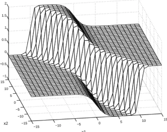
We illustrate this inuence with a simple experiment us- ing a MLP network with 2 input, 2 hidden, and 1 output unit. The target function is also dened by a parameter in this model (Fig.2). The normal distribution

(0

16

2 ) is used for

, where

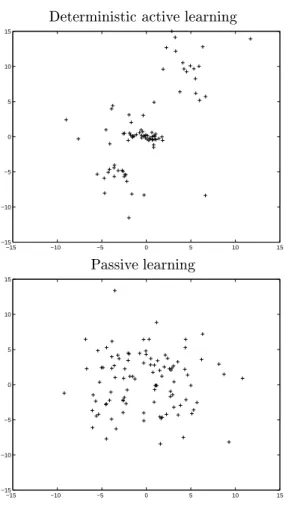
( m

) means the normal distribution with m as its mean and as its variance-covariance ma- trix. Fig.3 shows the average of generalization errors for 50 trials changing initial training data set. The result of de- terministic active learning is inferior to that of passive one after 60 data. We nd that the parameter sometimes does not approach to ^ because of the excessive localization of training data, which is shown clearly in Fig.4.

III. Probabilistic active learning A. Probabilistic active learning methods

We propose two probabilistic active learning methods.

One is the parametric active learning, which utilizes a para- metric probability family to generate a new input point.

−15 −10 −5 0 5 10 15

−15

−10

−5 0 5 10 15

−1

−0.5 0 0.5 1 1.5 2

x1 x2

Fig. 2. The true function of 2-2-1 MLP model

20 40 60 80 100 Number of training data

1E-03 1E-02 1E-01

Av. of generalization errors (50 trials)

Deterministic active learning Passive learninig

Fig. 3. Deterministic active learning

Deterministic active learning

−15 −10 −5 0 5 10 15

−15

−10

−5 0 5 10 15

Passive learning

−15 −10 −5 0 5 10 15

−15

−10

−5 0 5 10 15

Fig. 4. Distributions of input data

This is a slight renement of the method proposed by Fukumizu ([17]). The other is the multi-point-search active learning, which generates a nite number of input points as candidates and selects the best one. In both methods, we introduce randomness which is expected to solve the problem of excessive localization.

A.1 Parametric active learning

Instead of optimizing a point x in eq.(10), we introduce a parametric family of the density functions

( x ^; v ⁾

^for

generating x , and try to optimize the density. A possible choice of

( x ^; v ⁾

is a normal mixture model dened by

r

( x ^; v ^{) = X}

k

=

c

(

)

exp

2 2

k

k

x

m

⁽¹²⁾

where

0 (

= 1

), ^P

₌₁

= 1, and v ⁼

(

m

m

) is a variable parameter vec- tor. Since a normal mixture converges to a point distribu- tion if

goes to zero, we should restrict the value of

in [

) for a positive

.

We optimize the density by nding the best v ^{to mini-}

mize

Tr

(^

^{1 )}

^{(^}

^{1 ;}

^{1 ) +}

^{(^}

^{1 ;}

⁾

¹

⁽¹³⁾

where

J

( ^;

^{) = Z}

^{( ;} x ⁾

⁽ x ^; v ⁾

x

⁽¹⁴⁾

The algorithm is described as follows.

[PARAMETRIC ACTIVE LEARNING]

1

. Prepare an initial set of training data

.

2

. Calculate the initial estimator ^

with respect to

.

3

. Prepare an initial parameter v

^.

4

.

:=

0 + 1.

5

. Find v

that minimizes

Tr

(^

^{1 )}

^{(^}

^{1 ;}

^{1 ) +}

^{(^}

^{1 ;}

⁾

¹

using a numerical optimization method.

6

. Generate an input data x ⁽

^{) from}

⁽ x ^; v

^).

7

. Feed x ⁽

⁾ to the target system. Observe a response y ⁽

^{) .}

8

. Set

:=

1

( x ⁽

⁾

y ⁽

^{) ).}

9

. Calculate the LSE estimator ^

with respect to

.

10

.

:=

+ 1.

11

. if

, then END, otherwise go to

.

Although the selected data are optimal only probabilisti- cally at best, they distribute over the input space more widely than those of deterministic active learning. we can expect this prevents the excessive localization of training data. However, this method needs the integral calculation of

(^

^{1 ;}

) in each iteration of numerical optimization.

The calculation cost is very expensive.

A.2 Multi-point-search active learning

We consider a method in which multiple candidates of the next point are generated and the best one that mini- mizes

Tr ^h

(^

^{1 )}

^{1 (^}

^{1 ;}

¹

x

^{) i}

is selected. If the number of candidates increases according to the number of training data, the best one converges to the true optimal location. This method is more random in early stage of the training, and it comes to generate the optimal data gradually. It aims at avoiding local minima for a small number of training data. Learning in early stage is especially important, because it is very dicult to converge to

if data are generated based on a wrong estimate of ⁰ . If we generate random candidates subject to

, the learning moves from passive to active.

The algorithm is described as follows. The number of candidates for the

th training data,

, is an increasing function of

.

[MULTI-POINT-SEARCH ACTIVE LEARNING]

1

. Prepare an initial set of training data

.

2

. Calculate the initial estimator ^

with respect to

.

3

.

:=

0 + 1.

4

. Generate

input data x

x

^{. Choose} x ⁽

⁾ according to

x ⁽

^{) = arg min}

<j>

Tr ^h

(^

⁾

^{(^}

^;

x

^{) i}

5

. Feed x ⁽

⁾ to the target system. Observe a response y ⁽

^{) .}

6

. Set

:=

1

( x ⁽

⁾

y ⁽

^{) )}

^.

7

. Calculate the LSE estimator ^

with respect to

.

8

.

:=

+ 1.

9

. if

, then END, otherwise go to

.

This method does not require numerical minimization.

This remarkably saves the computational cost, which is often a problem of active learning methods.

B. Comparison with other active learning methods There have been proposed other active learning methods which use Fisher information matrixes. We briey review them and compare them with ours.

The most famous criterion of experimental design is D- optimality ([1]), which selects input data that maximize det

( ⁰

). It is known ([18]) that under some condi- tions D-optimality is equivalent to the minimax criterion that selects the input data

according to

min

X

N

max

x

E ^h

f ⁽ x ^{; ^ )}

f ⁽ x ^;

⁾

ⁱ

⁽¹⁵⁾

In a sequential implementation of D-optimality ([1]), the selected point attains the maximum of the expected vari- ance of the estimation dened by

V

( x ^{) = E h}

y

f ⁽ x ^{; ^ )}

ⁱ

⁽¹⁶⁾

Kindermann et al. ([19]) proposes an active learning method for neural networks based on this criterion. They use the bootstrap to estimate

( x ). The computational cost of this method is very expensive, since we have to per- form both the bootstrap and the numerical optimization of the input point.

These criterions are clearly dierent from ours in that they do not minimize the generalization error. It depends on the purpose of learning which criterion should be ap- plied.

Cohn ([4]) proposes a method that uses reference points to avoid the integral calculation of

( ). He uses a ran- dom reference point x

, and selects the next point that minimizes

Tr ^h

( x

^{; ^}

⁾

^{(^}

^;

x

^{) i}

⁽¹⁷⁾

Although our methods look similar to this, they are essen- tially dierent in that the objective of our method is to minimize the generalization error. Note that the above cri- terion is dierent from eq.(10) even if x

is taken from

, because the operations of min and integral are not change- able. However, we can expect that this method also has an eect of avoiding localization of input points by the varia- tion of reference points.

C. Experimental results on active learning methods We show simple experimental results to compare the per- formance and property of active learning methods.

The rst experiment is a very simple one to see the basic properties of various active learning methods. We use the MLP model with 1 input, 1 hidden, and 1 output unit. The target function is given by

f

( x ^{) =}

⁽ x ⁾

⁽¹⁸⁾

which is realized by the model. The total number of train- ing data is 100. The initial 10 data are given passively subject to

=

(0

1). The deviation of the noise added to the output is 0.1. We compare the following 5 methods;

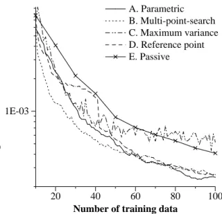
A. parametric active learning B. multi-point-search active learning C. maximum variance point ([19]) D. usage of reference points ([4]) E. passive learning

In method A, we use a mixture model of four normal dis- tributions. The candidates in method B are generated by

Q

, and

= ^lp 10(

10) ^m . In Method C, we use 20 bootstrap samples in estimating

( x ). In Method D, the probability to generate reference points is

.

Fig.5 shows the average of generalization errors for 50

sets of training data. Active learning with method A, B,

and D outperform passive learning. The proposed meth-

ods, A and B, show good performance in generalization er-

ror. Interestingly, method D is as good as A and B, though

the criterion does not precisely minimize the generalization

error. Method C also shows eectiveness in small number

of training data, while the nal result is worse than the result of passive learning. This is reasonable because the criterion of method C is dierent from minimization of the generalization error. In fact, there are many training data selected very far from the high-density region of

.

Next, we apply active learning methods to see the perfor- mances in a little complicated problem, which is the same as the one in Section II.C (Fig.2). We omit the method C in this simulation, since it is computationally very ex- pensive and we know from the previous experiment that the performance in the generalization error is not so high.

Fig.6 shows the average of generalization errors for 50 data sets. In this case, the multi-point-search method shows the best performance. Although parametric active learning still shows much better performance than passive learning, its eect is not so remarkable as the eect of the multi- point-search method. One reason is that the density model

r

( x ^; v ), which is the mixture of 4 normal distributions, is not sucient to express the optimal density. In fact, as we can see in Fig.7, the distribution of the input data in the parametric method is more concentrated around the center than the multi-point-search method. Although Method D shows eectiveness in early stage of learning, it is worse than passive learning after the number of data becomes large. This seems natural because the criterion is not equiv- alent to the generalization error.

In both simulations, our probabilistic active learning methods show signicant reduction of the generalization error. The multi-point-search method shows almost the best in both simulations. In the parametric method, we have to choose carefully a density family

( x ^; v ^{), which}

has an essential inuence on the performance. It is also a disadvantage of the parametric method that the deviation of data from the optimal position remains even after the training has converged successfully. On the other hand, in the multi-point-search method, we have only to choose the number of candidates at each sampling. It automati- cally increases the optimality of selected locations. Cohn's method also shows eectiveness in the generalization error in spite of the dierence of the criterion. However, in the latter simulation, the eect becomes comparatively small as the increase of the number of data.

IV. Model selection in active learning A. Model mismatch problem in active learning

In the previous sections, we assume that the true func- tion is completely included in the model or can be approx- imated by the model with high accuracy. This assumption is too strong in actual machine learning problems. On the other hand, it is easy to see that active learning does not work if the model has a large bias. The data set given by active learning is far from optimal, for example, if we es- timate a quadratic function by the linear regression model believing that the true function is linear.

Model selection is, then, especially important in active learning. It is known that a MLP can approximate any continuous function on a compact set with arbitrary ac- curacy ([20],[21],[22]). Therefore, a network with a su-

20 40 60 80 100

Number of training data 1E-03

Av. of generalization errors (50 trials)

A. Parametric B. Multi-point-search C. Maximum variance D. Reference point E. Passive

Fig. 5. Comparison of active learning methods (1-1-1)

20 40 60 80 100

Number of training data 1E-03

1E-02 1E-01

Av. of generalization errors (50 trials)

A. Parametric B. Multi-point-search D. Reference point E. Passive

Fig. 6. Comparison of active learning methods (2-2-1)

ciently large number of hidden units can almost realize the

true function. A network with many hidden units, how-

ever, causes a critical problem in active learning, in addi-

tion to the increase of the generalization error caused by

surplus parameters. It is proved that the Fisher informa-

tion matrix at the true parameter is singular if and only

if the model has surplus hidden units to realize the true

function ([12]). Even if the true function cannot be re-

alized perfectly, the Fisher information of a network with

almost redundant hidden units is very close to a singular

one, which makes an algorithm using the inverse matrix

numerically unstable. We should establish a method of

keeping the Fisher information matrix non-singular during

learning. We will describe a solution to this problem in

this section. This method is rst introduced in Fukumizu

Parametric method

−15 −10 −5 0 5 10 15

−15

−10

−5 0 5 10 15

Multi-point-search method

−15 −10 −5 0 5 10 15

−15

−10

−5 0 5 10 15

Fig. 7. Distributions of input data ([17]), and we give its full description here.

B. Pruning for regularity of a Fisher information matrix Our pruning technique is based on the following theorem.

Theorem 1 ([12]) The Fisher information matrix of a

three-layer perceptron at a parameter ^{= (}

¹¹

¹

¹¹

¹

⁾

is singular if and only if one of the following three condi- tions holds;

(1) there exists

such that u

^{:= (}

⁾

⁼ 0 ^.

(2) there exists

such that w

^{:= (}

⁾

⁼ 0 ^.

(3) there exist dierent

1 and

2 such that ( u

^{) =}

( u

^).

According to this theorem, we can keep the Fisher in- formation of a network non-singular by checking the above three conditions which indicate the existence of redundant hidden units, and by pruning them if any. The parameter should be modied in (1) and (3) to keep the function un- changed, when the redundant hidden unit is removed. The following is the pruning procedure. Note that we use the relation

(

) = 1

(

) in the derivation of (D). We write

H

j

for the

th hidden unit.

[Pruningprocedure]

(A) If u

⁼ 0 ^{, then}

[P1] eliminate

and

+

(

) for all

.

(B) If w

⁼ 0 ^{, then}

[P2] eliminate

.

(C) If ( u

^{) = (} u

^{), then}

[P3] eliminate

and

+

for all

. (D) If ( u

^{) =}

⁽ u

^{), then}

[P4] eliminate

and

,

+

for all

.

In most problems, there is little possibility that a Fisher information is perfectly singular. However, we should re- move almost redundant hidden units to ensure the stability of the inverse. At the same time, necessary hidden units should not be removed because it results in the increase of the model bias. We must establish a criterion to determine when hidden units should be removed.

We eliminate a hidden unit if the inequality

Z

k

f ⁽ x ^{; ~ )}

f ⁽ x ^{; ^ )}

N

(19) is satised for the LSE estimator ^ and a pruned estima- tor ~ derived from [P1]-[P4]. The constant

is a positive number. If there is no redundant hidden unit, it is known that the LSE estimator approaches to

in the order of

N

;

1

2 . The asymptotic behavior in the existence of re- dundant hidden units is very complicated and still an open problem. Therefore, we put an assumption

E ^Z

f ⁽ x ^{; ^ )}

f ⁽ x ^;

⁾

⁽ x ^{) =}

⁽

^{1 )}

⁽²⁰⁾

and use eq.(19) as heuristics.

We employ a pruning procedure during the batch back- propagation algorithm, in which one training example in a xed data set is used for one update of the parameter.

The condition of eq.(19) is checked for every candidate of a pruned estimator ~ ^{once in}

updates. Eq.(19) can be satised during the training if the optimal parameter ^{0 is}

located within the order of

¹

² distance of the parame- ter set that realizes networks with redundant hidden units, Therefore, the following pruning algorithm is expected to eliminate only almost redundant hidden units. The condi- tions in (a)-(d) are derived by calculating eq.(19). In the following, we write ^

for

(^ u

x ^{+ ^}

^).

[BP with hiddenunitpruning]

1

.

:= 1.

2

. Update ^ with respect to ( x ⁽

^mod

⁾

y ⁽

^mod

^{) ) using}

the back-propagation rule.

3

. If

mod

= 0, then execute the following four sub- procedure:

(a) If

w ^

^{2 Z (^}

^{(^}

^{)) 2}

⁽ x ⁾

, then execute [P1].

(b) If

w ^

^{2 Z (^}

^{) 2}

⁽ x ⁾

, then execute [P2].

(c) If

w ^

^{2 Z (^}

^{^}

^{) 2}

⁽ x ⁾

^for

¹

⁼

^{2 ,}

then execute [P3].

(d) If

w ^

^{2 Z (1}

^{^}

^{^}

^{) 2}

⁽ x ⁾

^for

¹

⁼

j

2 , then execute [P4].

4

.

:=

+ 1.

5

. If

, then END. Otherwise go to

.

A positive constant

and a natural number

control the possibility of pruning. The constant

should be su- ciently large so that the inverse of a Fisher information matrix can be stably calculated. On the other hand,

should be small enough for the pruning procedure to pre- serve eliminate necessary hidden units. The optimization of these values is also very dicult, because it requires to know the exact asymptotic behavior of the estimator in the existence of redundant hidden units. Therefore, we decide them heuristically in this paper.

C. Active learning with hidden unit pruning

The pruning procedure keeps the information matrix nonsingular and makes the active learning methods appli- cable to a MLP even if we rst prepare a surplus number of hidden units. The modication of active learning methods is simple. We have only to use the BP with hidden unit pruning instead of the usual back-propagation.

We demonstrate the eect of the modied methods through experiments in which the true function is not in- cluded in the MLP model. We use the MLP model with 4 input units, 7 hidden units, and 1 output unit. The true function is given by

f

( x ^{) = erf(}

⁾

where x ^{= (}

^{) and erf(}

) is the error function dened by

erf(

) = ^r 2

Z

0

;x 2

dx:

The graph of the error function resembles that of the sig- moidal function, while they never coincide by any ane transforms. The model has many almost redundant hid- den units in this case. We set

=

(0

9

4 ). The nal number of training data is 300. The deviation of the noise added to the output is 0.01. In the parametric active learn- ing method, the mixture model of 5 normal distributions is used for

( x ^; v ). To save the computational cost, we gener- ate 5 data at one time. When new data are generated, all data are presented 50000 times cyclically in the BP train- ing, and the pruning conditions are checked every 100 up- dates of parameters from 40000th through 50000th cycle.

In the multi-point-search active learning,

candidates are generated for selecting

th training data. In this case, all the data are presented 5000 times cyclically each time a new data is added, and the pruning condition is checked every 100 updates from 4000th through 5000th cycle.

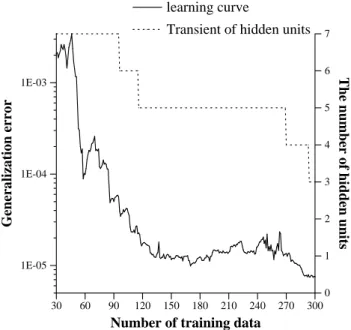
Fig.8 shows the average of generalization errors for 10 sets of training data. We nd that the active learning methods reduce the error remarkably, though the bias-free assumption is not satised. Fig.9 shows a typical learning

30 60 90 120 150 180 210 240 270 300

Number of training data

1E-05 1E-04 1E-03

Av. of generalization errors (10 trials)

parametric multi-point-search passive

Fig. 8. Active/Passive learning :

(

) = erf(

).

30 60 90 120 150 180 210 240 270 300

Number of training data

1E-05 1E-04 1E-03

Generalization error

learning curve

0 1 2 3 4 5 6 7

The number of hidden units

Transient of hidden units

Fig. 9. A typical learning curve of multi-point-search active learning.

curve of the multi-point-search method, and the transition of the number of hidden units during the learning. We see the elimination of redundant hidden units. The general- ization error is reduced by both the eect of pruning and active learning.

V. Application to a color conversion problem

We apply our active learning methods with the pruning

technique for a color conversion problem, which is found in

many color reproduction systems using CMY (cyan, ma-

genta, and yellow) ink. The problem is to simulate a spe-

cic color reproduction system like a color printer, which

produces a color print for a given CMY input signal. The

print result can be physically measured and represented by

a color system like RGB. It is very important to know the function from CMY to RGB of a specic system to achieve accurate color reproduction. It is known that the func- tion from CMY to RGB can be theoretically given by the Neugebauer equations ([23]). However, a practical system like a color xerography has a very complicated mechanism, and the theoretical equations cannot predict the actual re- sult with high accuracy. The neural network approach is one of the methods to approximate the non-linear relation of the color conversion ([24]). Moreover, since the precise measurement of color is costly, active learning is a promis- ing way to simulate the system.

In this paper, to demonstrate the eectiveness of our active learning methods, we estimate the relation of the Neugebauer equations instead of using a real color repro- duction system. It is known that the Neugebauer equations approximate the real system well in the case of oset print- ing. Then, if we can verify eectiveness in estimating the theoretical equations, we can also expect the eectiveness in approximating a real system.

The model which we use has 3 input and 3 output units.

The initial number of hidden units is 8. For the param- eters of the Neugebauer equations, we use the relation in [25]. We add an independent Gaussian noise

(0

10

⁴

3 ) to the output of the Neugebauer equations to simulate a measurement noise. Since we have no meaningful reason to assume a special environmental distribution, we use the uniform distribution on [0

1] ³ for

. After the initial train- ing with 30 examples which are given passively, we train a network by the parametric and multi-point-search active learning method, collecting training samples one by one up to 150. In the parametric method, we use a mixture model of 8 normal distributions restricted on [0

1] ³ . In the multi-point-search method, the number of candidates is ^lp 10(

30) ^m .

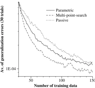
Fig.10 shows the average of generalization errors for 30 trials with dierent initial training examples. We can see the results of the active learning methods remarkably out- perform the result of passive learning. If we evaluate their eect by

(

)

(

), where

(

) and

(

) are the value of the graphs at

th data for parametric ac- tive learning and passive learning respectively, the aver- age of

(

)

(

) for

= 50

100 is 0.80, and the average for

= 50

150 is 0.85. The eect of the multi-point-search method in the same manner is 0.61 for

i

= 50

100, and 0.67 for

= 50

150. These results clearly show the eectiveness of our methods in this real- world application. The multi-point-search method shows a better result than the parametric method throughout the training, and the advantage of the latter method over pas- sive learning is smaller at the nal stage of learning. One of the reasons of this is the probabilistic aspect as described in Section IV. Especially, it is dicult to nd a suitable den- sity family on a compact input space. This problem always arises if the input space is bounded, and is a disadvantage of the parametric method.

50 100 150

Number of training data 1E-04

Av. of generalization errors (30 trials)

Parametric Multi-point-search Passive

Fig. 10. Active learning of a color conversion problem

VI. Conclusion

We discussed statistical active learning methods for the purpose of applying them to the multilayer perceptron model. We explained the problem of local minima in active learning of neural networks, and proposed two probabilis- tic active learning methods to prevent local minima. This problem does not appear in linear models, in which the least square error estimator can be solved directly.

We explained the importance of model selection espe- cially in active learning. The derivation of many active learning methods requires that the model includes the true function. This is essential to the eect of active learning, while we cannot assure it in many practical applications.

On the other hand, too many hidden units make the active learning methods inapplicable because of the singularity of Fisher information matrixes. To solve this problem, we proposed the active learning method with pruning to keep the Fisher information nonsingular, based on the theorem that claries the singularity condition of a Fisher infor- mation matrix of a three-layer perceptron. Experimental results showed that active learning with pruning eliminated surplus hidden units and had a remarkable eect of reduc- ing the generalization error.

Acknowledgments

The author would like to express gratitude to Dr. Sumio

Watanabe for his encouragement and helpful comments.

References

[1] V.V. Fedorov. Theory of Optimal Experiments . Academic Press, New York, 1972.

[2] R.H. Myers, A.I. Khuri, and W.H. Carter, Jr. Response surface methodology: 1966-1988. Technometrics , 31(2):137{157, 1989.

[3] D. MacKay. Information-based objective functions for active data selection. Neural Computation , 4(4):305{318, 1992.

[4] D.A. Cohn. Neural network exploration using optimal experi- ment. In J. Cowan et al., editor, Advances in Neural Information Processing Systems 6 , pages 679{686, San Meteo, 1994. Morgan Kaufmann.

[5] P. Sollich. Query construction, entropy and generalization in neural network models. Physical Review E , 49:4637{4651, 1994.

[6] K. Fukumizu and S. Watanabe. Error estimation and learning data arrangement for neural networks. In Proceedings of IEEE International Conference on Neural Networks , volume 2, pages 777{780, June 1994.

[7] H. Cramer. Mathematical method of statistics , pages 497{506.

Princeton University Press, Princeton, NJ, 1946.

[8] H. Akaike. A new look at the statistical model identication.

IEEE Trans. Automatic Control , 19(6):716{723, 1974.

[9] H. White. Learning in articial neural networks: a statistical perspective. Neural Computation , 1:425{464, 1989.

[10] N. Murata, S. Yoshizawa, and S. Amari. Network information criterion { determining the number of hidden units for an ar- ticial neural network model. IEEE Trans. Neural Networks , Vol.5, No.9:865{872, 1994.

[11] S. Watanabe and K. Fukumizu. Probabilistic design of layered neural networks based on their unied framework. IEEE Trans- action on Neural Networks , 6(3), 1995.

[12] K. Fukumizu. A regularity condition of the information matrix of a multilayer perceptron network. Neural Networks , Vol.9, No.5:871{879, 1996.

[13] B. Efron and R. Tibshirani. An introduction to the bootstrap . Chapman and Hall, New York, 1993.

[14] M. Stone. Cross-validatory choice and assessment of statistical predictions. J. Royal Statist. Soc. , 36:111-133, 1974.

[15] V.N. Vapnik. Estimation of dependences based on empirical data . Springer-Verlag, New York, 1982.

[16] J. Moody. The eective number of parameters: An analysis of generalization and regularization in nonlinear learning systems.

In Advances in Neural Information Processing Systems , [17] K. Fukumizu. Active learning in multilayer perceptrons. In

D. S. Touretzky et al., editor, Advances in Neural Information Processing Systems 8 , pages 295{301, Cambridge, 1996. MIT Press.

[18] J. Kiefer and J. Wolfowitz. The equivalence of two extremum problem. Canadian Journal of Mathematics , 12:363{366, 1960.

[19] J. Kindermann, G. Paass, and F. Weber. Query construction for neural networks using the bootstrap. In Proceedings of In- ternational Conference on Articial Neural Networks 95 , pages 135{140, 1995.

[20] G. Cybenco. Approximation by superpositions of a sig- moidal function. Mathematics of Control, Signals and Systems , 2(4):303{314, 1989.

[21] K. Funahashi. On the approximate realization of continuous mapping by neural networks. Neural Network , 2:183{192, 1989.

[22] K. Hornik, M. Stinchcombe, and H. White. Multi-layer feed- forward networks are universal approximators. Neural Networks , 2:359{366, 1989.

[23] H.E.J. Neugebauer. Die theoretishen Grundlagen des Mehrfar- ben buchdrucks. Zeitschrift fur wissenschaftliche Photographik, Photophysik, und Photochemie , 36(4):73{89, 1937.

[24] T. Iga, Y. Arai, and S. Usui. Trend of a present color management technology in the industry. In Proceedings of 5th International Conference on Neural Information Processing (ICONIP'98) , pages 40{43, 1998.

[25] J.A.C. Yule. Principles of color reproduction , Appendix E. John

Willey & Sons, New York, 1967.