R ESEARCH I NSTITUTEFOR M ATHEMATICAL S CIENCESKYOTOUNIVERSITY,Kyoto,Japan BySakieSUZUKINovember2011 Ontheuniversal sl invariantofBrunnianbottomtangles RIMS-1732

RIMS-1732

On the universal sl

2

invariant of Brunnian bottom tangles

By

Sakie SUZUKI

November 2011

R _ESEARCH I NSTITUTE FOR M ATHEMATICAL S _CIENCES

On the universal sl ₂ invariant of Brunnian bottom tangles

Sakie Suzuki

November 27, 2011

Abstract

A linkL is called Brunnian if every proper sublink ofL is trivial. Similarly, a bottom tangleT is called Brunnian if every proper subtangle of T is trivial. In this paper, we give a small subalgebra of the n-fold completed tensor power of Uh(sl2) in which the universal sl2 invariant of n-component Brunnian bottom tangles takes values. As an application, we give a divisibility property of the colored Jones polynomial of Brunnian links.

1 Introduction

The universal invariant of tangles associated with a ribbon Hopf algebra [3, 5, 6, 7, 8, 9, 13, 14] has the universality property for the colored link invariants which are defined by Reshetikhin and Turaev [14].

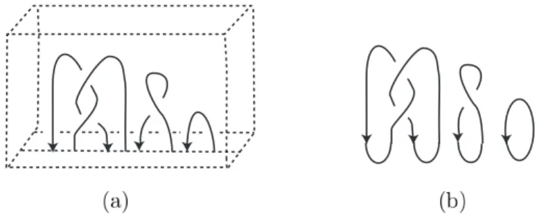
The universal sl2 invariantJT of an n-component bottom tangleT takes values in then-fold completed tensor powersUh(sl2)^⊗ˆnofUh(sl2), and we can obtain the colored Jones polynomial of the closure link cl(T) fromJT by taking the quantum traces. Here, abottom tangle is a tangle in a cube consisting of only arc components such that each boundary point is on the bottom and the two boundary points of each arc are adjacent to each other, see Figure 1 (a) for example. The closure of a bottom tangle is defined as in Figure 1 (b).

Our interest is in the relationship betweentopological properties of tangles and links andalgebraic propertiesof the universalsl2invariant and the colored Jones polynomial.

Habiro [3] proved that the universalsl2 invariant of n-component, algebraically-split, 0-framed bottom tangles takes values in a subalgebra ( ˜Uq^ev)^⊗˜n of Uh(sl2)^⊗ˆn (Theorem 4.4). The present author proved improvements of this result with a smaller subalgebra ( ¯U_q^ev)ˆ^⊗ˆn ⊂ ( ˜Uq^ev)^⊗˜n in the special case of ribbon bottom tangles [15] and boundary bottom tangles [16] (Theorem 4.5). Here, the result for boundary bottom tangles had been conjectured by Habiro [3].

∗Research Institute for Mathematical Sciences, Kyoto University, Kyoto, 606-8502, Japan. E-mail address:[email protected]

Figure 1: (a) A bottom tangleT, (b) The closure link cl(T) ofT

A link L is called Brunnian if every proper sublink of L is trivial. Similarly, a bottom tangleT is calledBrunnian if every proper subtangle of T is trivial, i.e., looks like ∩ · · · ∩. Habiro [4, Proposition 12] proved that for every Brunnian linkL, there is a Brunnian bottom tangle whose closure is isotopic toL.

In the present paper, we give a subalgebraU_Br⁽ⁿ⁾ofU_h(sl₂)^⊗ˆn such that ( ¯U_q^ev)ˆ^⊗ˆn⊂ U_Br⁽ⁿ⁾⊂( ˜Uq^ev)^⊗˜n in which the universal sl2 invariant of n-component Brunnian bottom tangles takes values (Theorem 4.7). As an application, we prove a divisibility property of the colored Jones polynomial of Brunnian links (Theorem 5.4).

The rest of this paper is organized as follows. In Section 2, we recall basic facts of the quantized enveloping algebraUh(sl2). In Section 3, we define the universalsl2invariant of bottom tangles. In Section 4, we give the main result for the universalsl2 invariant of Brunnian bottom tangles. In Section 5, we give an application for the colored Jones polynomial of Brunnian links. Section 6 is devoted to the proofs of the results.

2 Quantized enveloping algebra U

(sl

)

In this section, we recall the definition of Uh(sl2) and its subalgebras. We follow the notations in [3, 16].

2.1 Quantized enveloping algebra U

(sl

)

We recall the definition of the universal enveloping algebraU_h(sl₂).

We denote by Uh = Uh(sl2) the h-adically complete Q[[h]]-algebra, topologically generated byH, E,andF, defined by the relations

HE−EH = 2E, HF−F H =−2F, EF−F E= K−K⁻¹ q^1/2−q^−1/2, where we set

q= exph, K=q^H/2= exphH 2 .

We equip Uh with the topologicalZ-graded algebra structure such that degE = 1, degF =−1, and degH = 0. For a homogeneous element xof Uh, the degree of x is denoted by|x|.

2.2 Z [q, q

]-subalgebras of U

(sl

)

We recallZ[q, q⁻¹]-subalgebras ofU_hfrom [3, 16].

In what follows, we use the followingq-integer notations.

{i}q =qⁱ−1, {i}q,n={i}q{i−1}q· · · {i−n+ 1}q, {n}q! ={n}q,n, [i]_q ={i}q/{1}q, [n]_q! = [n]_q[n−1]_q· · ·[1]_q,

[i n ]

q

={i}q,n/{n}q!, fori∈Z, n≥0.

Set

E˜⁽ⁿ⁾= (q^−1/2E)ⁿ/[n]q!, F˜⁽ⁿ⁾=FⁿKⁿ/[n]q! ∈Uh, (1) e= (q^1/2−q^−1/2)E, f = (q−1)F K ∈U_h, (2) forn≥0.

LetU_Z,q⊂Uh denote theZ[q, q⁻¹]-subalgebra generated byK, K⁻¹,E˜⁽ⁿ⁾, and ˜F⁽ⁿ⁾ forn≥1, which is aZ[q, q⁻¹]-version of the Lusztig’s integral form (cf. [10, 15]).

LetUq ⊂U_Z,q denote theZ[q, q⁻¹]-subalgebra generated byK, K⁻¹, e, and ˜F⁽ⁿ⁾ for n≥1.

Let ¯Uq⊂ Uq denote theZ[q, q⁻¹]-subalgebra generated byK, K⁻¹, eandf, which is aZ[q, q⁻¹]-version of the integral form defined by De Concini and Procesi (cf. [1, 15]).

For X = U_Z,q, Uq, ¯Uq, let X^ev denote the Z[q, q⁻¹]-subalgebra of Uh defined by the same generators asX except that K^±2 replacesK^±1, i.e.,U_Z^ev_,q ⊂U_Z,q denotes the Z[q, q⁻¹]-subalgebra generated by K², K⁻²,E˜⁽ⁿ⁾, ˜F⁽ⁿ⁾, n ≥ 1; Uq^ev ⊂ Uq denotes the Z[q, q⁻¹]-subalgebra generated by K², K⁻², e, ˜F⁽ⁿ⁾, n≥1; and ¯U_q^ev ⊂U¯q denotes the Z[q, q⁻¹]-subalgebra generated byK², K⁻², e,f.

To summarize, we have the following inclusions of the subalgebras ofUh. U¯_q^ev ⊂ Uq^ev ⊂ U_Z^ev_,q

∩ ∩ ∩

U¯_q ⊂ Uq ⊂ U_Z,q ⊂ U_h

2.3 Completion

In this section, we recall from [3] the completion ˜Uq^ev of Uq^ev in U_h and its completed tensor powers ( ˜Uq^ev)^⊗˜n forn≥0.

First, we define ˜Uq^ev. Forp≥0, letFp(Uq^ev) be the two-sided ideal inUq^ev generated bye^p. Let ˜Uq^evbe the completion ofUq^evin Uh with respect to the decreasing filtration {Fp(Uq^ev)}p≥0, i.e., we define ˜Uq^evas the image of the homomorphism

lim←−

p≥0

Uq^ev/Fp(Uq^ev)→Uh

induced byUq^ev⊂Uh.

We define ( ˜Uq^ev)^⊗˜n forn≥0. Forn= 0, we define ( ˜Uq^ev)^⊗˜0 =Z[q, q⁻¹]. Forn≥1, we define ( ˜Uq^ev)^⊗˜n as the completion of (Uq^ev)^⊗n in U_h^⊗ˆn with respect to the decreasing filtration{Fp

((Uq^ev)^⊗n)

}p≥0, where we set Fp

((Uq^ev)^⊗n)

=

∑n

i=1

(Uq^ev)^⊗(i−1)⊗ Fp(Uq^ev)⊗(Uq^ev)^⊗(n−i), p≥0, i.e., we define

( ˜Uq^ev)^⊗˜n= Im (

lim←−

p≥0

(Uq^ev)^⊗n/Fp

((Uq^ev)^⊗n)

→U_h^⊗ˆn )

.

For aZ[q, q⁻¹]-subalgebraAof (Uq^ev)^⊗n,n≥0, we denote by{A}ˆtheclosureofAin ( ˜Uq^ev)^⊗˜n, which is the completion ofA inU_h^⊗ˆn with respect to the decreasing filtration Fp

((Uq^ev)^⊗n)

∩A, i.e., {A}ˆ= Im

( lim←−

p≥0

(A/( Fp

((Uq^ev)^⊗n)

∩A)

→U_h^⊗ˆn )

.

In particular, we denoted by ( ¯U_q^ev)˜^⊗˜n the closure{( ¯U_q^ev)^⊗n}ˆof ( ¯U_q^ev)^⊗n in ( ˜Uq^ev)^⊗˜n.

3 Universal sl

invariant of bottom tangles

In this section, we recall the definition of the universalsl₂ invariant of bottom tangles.

3.1 Bottom tangles

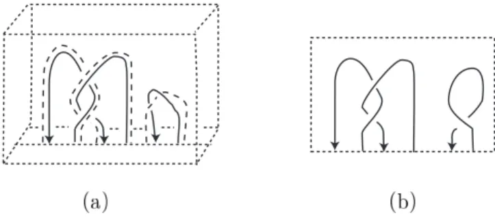
A bottom tangle (cf. [2, 3]) is an oriented, framed tangle in a cube consisting of arc components such that each boundary point is on a line on the bottom, and the two boundary points of each component are adjacent to each other. We give a preferred orientation of the tangle so that each component runs from its right boundary point to its left boundary point. For example, see Figure 2 (a), where the dotted lines represent the framing. We draw a diagram of a bottom tangle in a rectangle assuming the blackboard framing, see Figure 2 (b).

Theclosure linkcl(T) of a bottom tangleT is defined as the link inR³obtained from T by closing, see Figure 1 again. For eachn-component linkL, there is ann-component bottom tangle whose closure isL. For a bottom tangle, we can define its linking matrix as that of the closure link.

3.2 Universal R-matrix of U

Set

D=q^14H⊗H= exp(h

4H⊗H)

∈U_h^⊗ˆ2.

Figure 2: (a) A bottom tangle T, (b) a diagram ofT We use the followinguniversalR-matrix ofUh,

R^±1=∑

n≥0

α^±_n ⊗β^±_n ∈U_h^⊗ˆ2,

where we set formally

αn⊗βn( =α⁺_n ⊗β_n⁺) =D (

q^12n(n−1)F˜⁽ⁿ⁾K⁻ⁿ⊗eⁿ )

, α⁻_n ⊗β_n⁻=D⁻¹

(

(−1)ⁿF˜⁽ⁿ⁾⊗K⁻ⁿeⁿ )

.

(Note that the right hand sides are sums of infinitely many tensors of the formx⊗y withx, y∈Uh. We denote them byα^±_n ⊗β_n^± for simplicity.)

3.3 Universal sl

invariant of bottom tangles

For ann-component bottom tangleT =T₁∪· · ·∪T_n, we define the universalsl₂invariant J_T ∈U_h^⊗ˆn in four steps as follows. We follow the notation in [16].

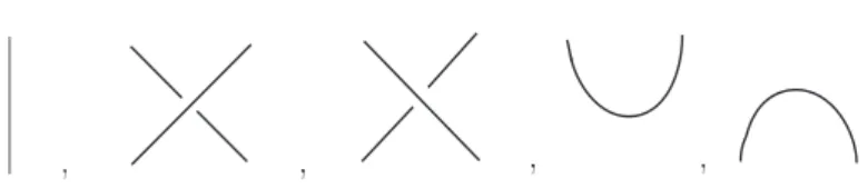
Step 1. Choose a diagram. We choose a diagram ˜T ofTobtained from the copies of the fundamental tangles depicted in Figure 3, by pasting horizontally and vertically.

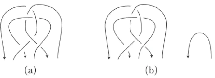
We denote byC( ˜T) the set of the crossings of ˜T. For example, for the bottom tangle B depicted in Figure 4 (a), we can take a diagram ˜B withC( ˜B) ={c1, c2}as depicted in Figure 4 (b). We call a map

s: C( ˜T) → {0,1,2, . . .} astate. We denote byS( ˜T) the set of states of the diagram.

Step 2. Attach labels. Given a states∈ S( ˜T), we attach labels on the copies of the fundamental tangles in the diagram following the rule described in Figure 5, where

“S^′” should be replaced with id if the string is oriented downward, and withSotherwise.

For example, for a statet∈ S( ˜B), we put labels on ˜B as in Figure 4 (c), where we set m=t(c1) andn=t(c2).

Step 3. Read the labels. We read the labels we have just put on ˜T and define an elementJT ,s˜ ∈U_h^⊗ˆn as follows. Let ˜T = ˜T1∪ · · · ∪T˜1, where ˜Ti corresponds to Ti. We

Figure 3: Fundamental tangles, where the orientations of the strands are arbitrary

Figure 4: (a) A bottom tangleB, (b) A diagram ˜B ofB, (c) The labels associated to a statet∈ S(B)

Figure 5: How to place labels on the fundamental tangles

define theith tensorand ofJT ,s˜ as the product of the labels on ˜Ti, where the labels are read off alongTi reversing the orientation, and written from left to right. For example, for the bottom tangleB and the statet∈ S( ˜B) in Figure 4, we have

JB,t˜ =S(α_m)S(β_n)⊗α_nβ_m.

Here, we identify the labelsS^′(α^±_i ) andS^′(β_i^±) with the first and the second tensorands, respectively, of the element S^′(α^±_i )⊗S^′(β_i^±) ∈ U_h^⊗ˆ2. Also we identify the label K^±1 with the elementK^±1∈Uh. ThusJT ,s˜ is a well-defined element inU_h^⊗ˆn. For example, we have

JB,t˜ =S(αm)S(βn)⊗αnβm

=∑

q^12m(m−1)q^12n(n−1)S(D^′₁F˜^(m)K^−m)S(D₂^′′eⁿ)⊗D^′₂F˜⁽ⁿ⁾K⁻ⁿD^′′₁e^m

= (−1)^m+nq^−n+2mnD⁻²( ˜F^(m)K⁻²ⁿeⁿ⊗F˜⁽ⁿ⁾K^−2me^m)∈U_h^⊗ˆ2, where D = ∑

D^′₁⊗D^′′₁ = ∑

D^′₂⊗D₂^′′. Note that JT ,s˜ depends on the choice of the diagram.

Step 4. Take the state sum. Set J_T = ∑

s∈S( ˜T)

JT ,s˜ .

For example, we have J_B = ∑

t∈S( ˜B)

JB,t˜ = ∑

m,n≥0

(−1)^m+nq^−n+2mnD⁻²( ˜F^(m)K⁻²ⁿeⁿ⊗F˜⁽ⁿ⁾K^−2me^m).

As is well known [13],J_T does not depend on the choice of the diagram, and defines an isotopy invariant of bottom tangles.

4 Results for the universal sl

invariant of bottom tangles

In this section, we give the main result for the universalsl2invariant of Brunnian bottom tangles.

4.1 Universal sl

invariant of algebraically-split bottom tangles, ribbon bottom tangles and boundary bottom tangles

We recall several results for the value of the universalsl2 invariant of bottom tangles.

Recall the sequence of the subalgebras ¯U_q^ev⊂ Uq^ev⊂U_Z^ev_,q⊂Uh.

For ann-component bottom tangleT, let Lk(T) denote the linking matrix ofT. Set D˜^Lk(T)= ∏

1≤i≤n

K_i^mii ∏

1≤i≤j≤n

D_ij^2mij ∈U_h^⊗ˆn,

where,Ki= 1^⊗i−1⊗K⊗1^⊗n−i for 1≤i≤nand Dij=∑

1^⊗i−1⊗D^′⊗1^⊗j−i−1⊗D^′′⊗1^⊗n−j, Dkk=∑

1^⊗k−1⊗D^′D^′′⊗1^⊗n−k, for 1≤i < j≤n, 1≤k≤n, whereD=∑

D^′⊗D^′′.

Theorem 4.1 ([15, Proposition 4.2, Remark 4.7]). Let T be an n-component bottom tangle. For every diagramT˜ ofT and every states∈ S( ˜T), we have

JT ,s˜ ∈D˜^Lk(T)(Uq^ev)^⊗n.

More precisely, the proof of [15, Proposition 4.2] implies the following.

Proposition 4.2. Let T be an n-component bottom tangle. For any diagram T˜ and any states∈ S( ˜T), we have

JT ,s˜ ∈D˜^Lk(T)F_|s|((Uq^ev)^⊗n), where we set|s|= max{s(c)| c∈C( ˜T)}.

Theorem 4.1 and Proposition 4.2 imply the following.

Theorem 4.3 ([15, Proposition 4.2, Remark 4.7]). For ann-component bottom tangle T, we have

JT ∈D˜^Lk(T)( ˜Uq^ev)^⊗˜n.

The following is the special case of Theorem 4.3 for algebraically-split bottom tangle with 0-framing (i.e., a bottom tangle with 0-linking matrix), which was proved first by Habiro [3].

Theorem 4.4 (Habiro [3]). Let T be an n-component algebraically-split bottom tangle with0-framing. Then we have

J_T ∈( ˜Uq^ev)^⊗˜n.

In [15] and [16], we defined a refined completion ( ¯U_q^ev)ˆ^⊗ˆn ⊂( ¯U_q^ev)˜^⊗˜n, and proved the following theorem, which is an improvement of Theorem 4.4 in the case of ribbon bottom tangles and boundary bottom tangles.

Theorem 4.5 ([15, 16]). Let T be an n-component ribbon or boundary bottom tangle with0-framing. Then we have

JT ∈( ¯U_q^ev)ˆ^⊗ˆn.

Remark 4.6. Theorem 4.5 with ( ¯U_q^ev)˜^⊗˜nreplaced with ( ¯U_q^ev)ˆ^⊗ˆnfor boundary bottom tangles had been conjectured by Habiro [3, Conjecture 8.9]. Here, we do not know whether the inclusion ( ¯U_q^ev)ˆ^⊗ˆn ⊂ ( ¯U_q^ev) ˜^⊗˜n is proper or not, but the definition of ( ¯U_q^ev)ˆ^⊗ˆn is more natural than that of ( ¯U_q^ev)˜^⊗˜n in the settings in [15, 16].

4.2 Result for the universal sl

invariant of Brunnian bottom tangles

The main result of this paper is the following, which is an improvement of Theorem 4.4 in the case of Brunnian bottom tangles.

Theorem 4.7. LetT be ann-component Brunnian bottom tangle withn≥3. We have JT ∈U_Br⁽ⁿ⁾,

where we set

U_Br⁽ⁿ⁾=

∩n

i=1

{(

( ¯U_q^ev)^⊗i−1⊗U_Z^ev_,q⊗( ¯U_q^ev)^⊗n−i

)∩(Uq^ev)^⊗n }

ˆ.

Here, since a trivial bottom tangle has 0-framing, a Brunnian bottom tangle also has 0-framing by the definition. To compare Theorem 4.7 with Theorems 4.4 and 4.5, forn≥3, we have the following.

{n-comp. alg. split bottom tangles with 0-framing} →^J ( ˜Uq^ev)^⊗˜n

∪ ∪

{n-comp. Brunnian bottom tangles} →^J U_Br⁽ⁿ⁾

∪ {n-comp. ribbon or boundary bottom tangles with 0-framing} →^J ( ¯U_q^ev)ˆ^⊗ˆn We can define the Milnor µ invariants [11, 12] of a bottom tangle as that of the corresponding string link described in [2, Section 13]. It is known that the Milnor µ invariants of ribbon bottom tangles and boundary bottom tangles vanish. It is also known that the Milnorµinvariants of length≤n−1 ofn-component Brunnian bottom tangles vanish. Thus we have the following conjecture.

Conjecture 4.8. (i) Let T be ann-component bottom tangle with0-framing. If the Milnor µinvariants ofT vanish, then we haveJT ∈( ¯U_q^ev)ˆ^⊗ˆn.

(ii) For n≥3, let T be an n-component bottom tangle with0-framing. If the Milnor µinvariants of T of length ≤n−1vanish, then we haveJ_T ∈U_Br⁽ⁿ⁾.

Theorem 4.7 is derived from the following proposition, which we prove in Section 6.1.

Proposition 4.9. Let T be an n-component Brunnian bottom tangle with n≥3. For eachi= 1, . . . , n, there is a diagram T˜⁽ⁱ⁾ of T such that

JT˜⁽ⁱ⁾,s∈( ¯U_q^ev)^⊗i−1⊗U_Z^ev_,q⊗( ¯U_q^ev)^⊗n−i for any states∈ S( ˜T⁽ⁱ⁾).

Figure 6: (a) The Borromean bottom tangleTB, (b) A bottom tangleT_B^′ Proof of Theorem 4.7 by assuming Proposition 4.9. For eachi= 1, . . . , n, by Theorem 4.7 and Proposition 4.2, there is a diagram ˜T⁽ⁱ⁾ ofT such that

JT˜⁽ⁱ⁾,s∈(

( ¯U_q^ev)^⊗i−1⊗U_Z^ev_,q⊗( ¯U_q^ev)^⊗n−i

)∩ F_|s|((Uq^ev)^⊗n)

for any states∈ S( ˜T⁽ⁱ⁾). Hence we have JT ∈{(

( ¯U_q^ev)^⊗i−1⊗U_Z^ev_,q⊗( ¯U_q^ev)^⊗n−i

)∩(Uq^ev)^⊗n }

ˆ for alli= 1, . . . , n.

Example 4.10. For the Borromean bottom tangleT_B depicted in Figure 6 (a), we have JT ∈{(

U_Z^ev_,q⊗( ¯U_q^ev)^⊗2

)∩(Uq^ev)^⊗3 }

ˆ

∩{(

U¯_q^ev⊗U_Z^ev_,q⊗U¯_q^ev

)∩(Uq^ev)^⊗3 }

ˆ

∩{(

( ¯U_q^ev)^⊗2⊗U_Z^ev_,q

)∩(Uq^ev)^⊗3 }

ˆ. See Example 6.2 for explicit expressions of JT.

Example 4.11. Let us add a trivial arc to the Borromean bottom tangle as in Fig- ure 6 (b), and denote it by T_B^′. Note that the bottom tangle T_B^′ is not Brunnian but algebraically-split. We have

J_T′

B=J_TB⊗1̸∈{(

( ¯U_q^ev)^⊗3⊗U_Z^ev_,q

)∩(Uq^ev)^⊗4 }

ˆ.

5 Application to the colored Jones polynomial

In this section, we give an application of Theorem 4.7 to the colored Jones polynomial of Brunnian links (Theorem 5.4).

5.1 Colored Jones polynomials of algebraically-split links, rib- bon links and boundary links

We recall results for the colored Jones polynomials of algebraically-split links, ribbon links, and boundary links.

For m≥1, let Vm denote the m-dimensional irreducible representation of Uh. Let Rdenote the representation ring of Uh overQ(q²¹), i.e.,Ris theQ(q¹²)-algebra

R= Span

Q(q¹2){V_m |m≥1}

with the multiplication induced by the tensor product. It is well known that R = Q(q¹²)[V2].

For an n-component link Lwith 0-framing, take a bottom tangle T whose closure isL. For X1, . . . , Xn ∈ R, the colored Jones polynomialJL;X₁,...,X_n of L with theith componentLi colored by Xi is given by

JL;X₁,...,X_n= (tr^X_q¹⊗ · · · ⊗tr_q^Xn)(JT)∈Q(q¹²), where, forY =∑

jyjVj∈ Randu∈Uh, we set tr^Y_q(u) = tr^Y(K⁻¹u) =∑

j

yjtr^Vj(K⁻¹u).

Habiro [3] studied the following elements inR Pl=

l−1

∏

i=0

(V2−qⁱ⁺¹² −q⁻ⁱ⁻¹²)∈ R, (3) P˜_l^′= q^12l

{l}q!Pl∈ R, (4)

forl≥0,which are used in an important technical step in his construction of the unified Witten-Reshetikhin-Turaev invariants for integral homology spheres.

Recall the notation{l}q,i ={l}q{l−1}q· · · {l−i+ 1}q for l ∈Z, i≥0. Theorem 4.4 implies the following.

Theorem 5.1 (Habiro [3]). Let L be an n-component algebraically-split link with 0- framing. Forl1, . . . , ln≥0, we have

J_{L; ˜P}′

l1,...,P˜_ln^′ ∈Z_a^(l1,...,ln). (5) Here we set

Z_a^(l1,...,ln)= {2lmax+ 1}q,l_max+1

{1}q

Z[q, q⁻¹], wherelmax= max(l1, . . . , ln).

For l ≥0, let Il denote the ideal in Z[q, q⁻¹] generated by {l−k}q!{k}q! for k = 0, . . . , l. Theorem 4.5 implies the following improvement of Theorem 5.1.

Theorem 5.2 ([15, 16]). Let L be an n-component ribbon or boundary link with 0- framing. Forl1, . . . , ln≥0, we have

J_{L; ˜P′}

l1,...,P˜^′

ln ∈Z_r,b^(l1,...,ln). (6)

Here we set

Z_r,b^(l1,...,ln)=( ∏

1≤i≤n,i̸=iM

Il_i

)·Z_a^(l1,...,ln)

= {2l_max+ 1}q,lmax+1

{1}q

∏

1≤i≤n,i̸=iM

I_li,

wherelmax= max(l1, . . . , ln)andiM is an integer such thatli_M =lmax. Form≥1, let Φ_m=∏

d|m(q^d−1)^µ(md)∈Z[q] denote themth cyclotomic polynomial, where∏

d|mdenotes the product over all positive divisors dofm, and µis the M¨obius function. Forr∈Q, we denote by⌊r⌋the largest integer smaller than or equal tor.

In [17], we study the idealIl and prove the following result, which we use later.

Proposition 5.3([17]). Forl≥0, the idealIl is the principal ideal generated by gl= ∏

m≥1

Φ^tm^l,m, (7)

where

t_l,m=

{⌊^l+1_m ⌋ −1 for1≤m≤l, 0 forl < m.

5.2 Result for the colored Jones polynomial of Brunnian links

The following is an application of Theorem 4.7 to the colored Jones polynomial of Brunnian links, which we prove in Section 6.2.

Theorem 5.4. Let Lbe ann-component Brunnian link withn≥3. Forl₁, . . . , l_n≥0, we have

J_{L; ˜P}′ l1,...,P˜^′

ln ∈Z_Br^(l1,...,ln). (8)

Here we set

Z_Br^(l1,...,ln)= {2lmax+ 1}q,l_max+1

{1}q{l_min}q!

∏

1≤i≤n,i̸=i_M,i_m

Il_i,

where l_max = max(l₁, . . . , l_n), l_min = min(l₁, . . . , l_n) and i_M, i_m, i_M ̸= i_m, are two integers such thatli_M =lmax,li_m =lmin, respectively.

Since a Brunnian linkLwithn≥3 components is algebraically-split with 0-framing, L satisfies both (5) and (8). Note that there is no inclusion which satisfies for all l1, . . . , ln ≥ 0 between Za^(l1,...,ln) and Z_Br^(l1,...,ln). For example, we have Za^(2,2,2,2) ̸⊂

Z_Br^(2,2,2,2) andZ_Br^(2,2,2,2)̸⊂Za^(2,2,2,2)since Z_a^(2,2,2,2)= {5}q,3

{1}q Z[q, q⁻¹]

= (q−1)²(q+ 1)(q²+q+ 1)(q²+ 1)(q⁴+q³+q²+q¹+ 1)Z[q, q⁻¹], Z_Br^(2,2,2,2)= {5}q,3

{1}q{2}q!{1}⁴qZ[q, q⁻¹]

= (q−1)⁴(q²+q+ 1)(q²+ 1)(q⁴+q³+q²+q¹+ 1)Z[q, q⁻¹].

Forl1, . . . , ln≥0, set

Z˜_Br^(l1,...,ln)=Z_a^(l1,...,ln)∩Z_Br^(l1,...,ln).

The above argument implies the following refinement of Theorem 5.4.

Theorem 5.5. Let Lbe ann-component Brunnian link withn≥3. Forl1, . . . , ln≥0, we have

J_{L; ˜P′}

l1,...,P˜^′

ln ∈Z˜_Br^(l1,...,ln). Forn≥3, we have

Z_r,b^(l1,...,ln)=( ∏

1≤i≤n,i̸=iM

Il_i

)·Z_a^(l1,...,ln)

=(

{lmin}q!Il_min

)·Z_Br^(l1,...,ln).

Thus, comparing Theorem 5.5 with Theorems 5.1 and 5.2, we have the following for n≥3.

{n-comp. alg. split links with 0-framing}

J_{∗; ˜P′}

l1,...,P′˜

−→ ln Za^(l1,...,ln)

∪ ∪

{n-comp. Brunnian links}

J_{∗; ˜P′}

l1,...,P′˜

−→ ln Z˜_Br^(l1,...,ln)

∪ {n-comp. ribbon or boundary links with 0-framing}

J_{∗; ˜P′}

l1,...,P˜′

−→ ln Z_r,b^(l1,...,ln)

Remark 5.6. By Proposition 5.3, the idealsZa^(l1,...,ln), Z_r,b^(l1,...,ln),Z_Br^(l1,...,ln)and ˜Z_Br^(l1,...,ln) are principal, each generated by a product of cyclotomic polynomials. See [17] for details and examples.

6 Proofs

In this section, we prove Proposition 4.9 and Theorem 5.4.

6.1 Proof of Proposition 4.9

We use the following lemma.

Lemma 6.1. Form≥0 andk, l∈Z, we have S^k(α^±_m)⊗S^l(β^±_m)∈D^±(−1)k+l(

(U_Z,q⊗U¯_q)∩( ¯U_q⊗U_Z,q)) , Proof. Form≥0, we have

αm⊗βm=D(

q^12m(m−1)F˜^(m)K^−m⊗e^m)

=D(

q^m(m−1)f^mK^−m⊗E˜^(m))

∈D(

(U_Z,q⊗U¯_q)∩( ¯U_q⊗U_Z,q)) ,

(9)

α⁻_m⊗β_m⁻ =D⁻¹(

(−1)^mF˜^(m)⊗K^−me^m)

=D⁻¹(

(−1)ⁿq^12m(m−1)f^m⊗K^−mE˜^(m))

∈D⁻¹(

(U_Z,q⊗U¯_q)∩( ¯U_q⊗U_Z,q)) .

(10)

Fork, l∈Z, we have

(S^k⊗S^l)(D^±1) =D^±(−1)k+l, (11)

(S^k⊗S^l)(

(U_Z,q⊗U¯q)∩( ¯Uq⊗U_Z,q))

= (U_Z,q⊗U¯q)∩( ¯Uq⊗U_Z,q). (12) Forx∈Uh homogeneous, we have

(x⊗1)D^±1=D^±1(x⊗K^∓|x|). (13) Now, (9)–(13) imply the assertion. For example, we have

S(α_m)⊗S(β_m) = (S⊗S)(α_m⊗β_m)

∈(S⊗S) (

D(

(U_Z,q⊗U¯q)∩( ¯Uq⊗U_Z,q)))

⊂(

(U_Z,q⊗U¯_q)∩( ¯U_q⊗U_Z,q)) D

=D(

(U_Z,q⊗U¯_q)∩( ¯U_q⊗U_Z,q)) .

Proof of Proposition 4.9. LetT =T1∪ · · · ∪Tn be ann-component Brunnian bottom tangle with n ≥ 3. We prove the assertion for i = 1, i.e., we prove that there is a diagram ˜T ofT such that

JT ,s˜ ∈U_Z^ev_,q⊗U¯_q^ev⊗U¯_q^ev⊗ · · · ⊗U¯_q^ev (14) for any states∈ S( ˜T). The other cases 2≤i≤nare similar.

Since T is Brunnian, the subtangle T2∪ · · · ∪Tn is trivial. ThusT has a diagram T˜= ˜T1∪T˜2∪ · · · ∪T˜n whose subdiagram ˜T2∪ · · · ∪T˜nhas no crossing. See Figure 7 for an example of such a diagram for the Borromean ringsTB.

We prove that ˜T satisfies (14). Note that ˜T has only two types of crossings as follows.

Figure 7: Borromean ringsT_B and its diagramP =P₁∪P₂∪P₃ such thatP₂∪P₃ has no crossing

Figure 8: The labels on a crossing Type A: Crossings between ˜T1 and ˜T2∪ · · · ∪T˜n

Type B: Self crossings of ˜T₁

Recall from the definition ofJT ,s˜ in Section 3.3 the labels which are put on the diagram.

For the crossings of type A, by Lemma 6.1, we can assume that the labels on ˜T₁are legs of copies ofD^±1and elements ofU_Z,q, and the labels on ˜T2∪ · · · ∪T˜n are legs of copies ofD^±1 and elements of ¯Uq. For the crossings of type B, we assume that the labels on T˜1 are legs of copies ofD^±1 and elements ofU_Z,q. See Figure 8 for example, where⋄s denote elements inU_Z,q and◦s denote elements in ¯U_q.

Now, except copies of D^±1, all labels on ˜T1 are elements of U_Z,q, and all labels on T˜2∪ · · · ∪T˜n are elements of ¯Uq, see Figure 9 for example. We gather every copy ofD^±1

Figure 9: Labels exceptD^±1s, where the black dots areK^±1