情報処理学会研究報告 IPSJ SIG Technical Report Vol.2014-HPC-144 No /5/ CRS 2 CRS Performance evaluation of exclusive version of preconditioned ite

密行列専用のプレコンディショニングつき

反復法の性能評価

岩里 洸介

1

藤野 清次

2

高橋 康人

3

概要：反復法の行列ベクトル積の計算において，疎行列の非零要素のみを格納し，間接参照によりその計

算を行うことが多い．このような

CRS

形式は，必要メモリ量が少なくかつ計算量も必要最少限で抑えら

れることから，疎行列向き格納法の一つであるとされる．一方，密行列に対しては，ごく自然な発想とし

て，全ての要素を格納する

2

次元配列を使用すれば，直接参照による計算時間の短縮が図れる可能性があ

る．本論文では，密行列専用版として直接参照を用いる反復法を実装し，密行列専用版反復法がどの程度

高速化が図れるかを調べることにする．

キーワード：密行列，反復法，

CRS

形式

Performance evaluation of exclusive version of

preconditioned iterative method for dense matrix

Abstract: As well known, only nonzero entries of a sparse matrix are stored in memory in CRS format. In

this case, nonzero entries are refered using indirect access, because it requires a small amount of memory

and short time of computation. CRS format, however, is inefficient in case of dense matrix because direct

access can be done using two-dimensional array. In this article, we implement an exclusive version of iterative

methods with two-dimensional array for dense matrix. Through numerical experiments, we examine speedup

of computation time of the proposed version.

Keywords: Dense matrix, Iterative method, CRS format

1.

はじめに

連立一次方程式

Ax = b

を解くことを考える．ここで，

A

は非対称の係数行列，

x

は解ベクトル，

b

は右辺項ベ

クトルである．係数行列

A

が疎であるとき，行列要素は

CRS(Compressed Row Storage)

方式などを用いて非零要

素のみ格納される．このような手法は間接参照を用いて非

零要素のみ計算するため，要求されるメモリ量や計算量が

抑えられ，疎行列に対して効率がよいとされる

[3]

．一方，

密行列に対しては間接参照の回数が増加するため，効率が

良いとは限らない．自然な考えとして，密行列に対しては

Graduate School of Information Science and Electrical

En-gineering, Kyushu University

2 _{九州大学情報基盤研究開発センター}

Research Institute for Information Technology, Kyushu

Uni-versity

3 _{同志社大学理工学部}

Faculty of Science and Engineering, Doshisha University

全ての要素を

2

次元配列に格納し，直接参照を用いて計算

する方法が挙げられる

[3]

．

前処理において，係数行列が密行列である場合，行列ベ

クトル積の計算に要する計算量が増加する

[4]

．そのため，

行列ベクトル積

2

回分の計算量を必要とする

ILU(0)

前処

理ではなく行列ベクトル積

1

回分とスカラーベクトル積

2

回分の計算量が必要な

Eisenstat

版

SSOR

前処理

[11]

が密

行列に対して有効だと考えられる．

そこで，本論文では密行列専用版

(exclusive version)

の

解法として行列要素を全て

2

次元配列に格納し，直接参照

を用いて計算を行う反復法を実装した．さらに，数値実験

を通して，

Eisenstat

版

SSOR

前処理付きの従来版と密行

列専用版の解法を比較し，密行列専用版の解法の計算時間

における高速化の度合いを調査する．

本論文の構成は以下の通りである．第

2

節で，

Eisensatat

版

SSOR

前処理について述べる．第

3

節で，行列要素の格

納方法について記述し，前進後退代入における実装方法の

違いを示す．第

4

節で，密行列専用版反復法の高速化の度

合いを数値実験により調査し，第

5

節で，まとめを行う．

2.

Eisenstat

版 SSOR 前処理

密行列に対して有効な前処理を考える．前処理行列

M

を用いて

M

Ax = M

b

と変形させる．

ILU(0)

などの

前処理では，前処理を行うことにより行列ベクトル積の計

算

2

回分の計算量が必要となる．一方，

Eisenstat

版

SSOR

前処理

(

以下，

E-SSOR

前処理と表記

)[11]

で必要な計算量

は行列ベクトル積

1

回とスカラーベクトル積

2

回分であ

る．

E-SSOR

前処理は

ILU(0)

前処理よりも計算量が少な

いため，密行列に対して有効であると考えられる

[7]

．した

がって，本論文では

E-SSOR

前処理を適用する．

2.1

SSOR

前処理

まず，

SSOR

前処理

[2]

について述べる．

SSOR

前処理

では，係数行列を

A = L + D + U

と分離して得られる行

列を用いて，前処理行列

K

を

K = (L + D/ω)(D/ω)

(U + D/ω)

(1)

とする．ここで，

ω

は緩和係数を意味する．両側前処理後

の係数行列を

A

˜

，解ベクトルを

x

˜

，右辺項を

b

˜

とすると，

˜

A = (L + D/ω)

A(U + D/ω)

(D/ω),

(2)

˜

x = (D/ω)

(U + D/ω)x,

(3)

˜

b = (L + D/ω)

b

(4)

で あ る ．ま た ，反 復

k

回 目 に お け る 前 処 理 後 の 残 差

r

:= b

− Ax

を

r

˜

とすると，

˜

r

= ˜

b

− ˜

A˜

x

= (L + D/ω)

b

− (L + D/ω)

A

×

(U + D/ω)

(D/ω)(D/ω)

(U + D/ω)x

= (L + D/ω)(b

− Ax

)

= (L + D/ω)

r

(5)

と表される．

2.2

Eisenstat trick

SSOR

前処理は

Eisenstat trick

と呼ばれる手法を用いて

実装することで計算量を削減できる

[9]

．式

(2)

を

˜

A = ((U + D/ω)

+(L + D/ω)

(I + (1

− 2/ω)D(U + D/ω)

))(D/ω)

(6)

と式変形し，行列ベクトル積

Av

˜

を以下の手順で計算す

る

[5][8]

．

1.

y = (U + D/ω)

(D/ω)v,

2.

z = (D/ω)v + (1

− 2/ω)Dy,

3.

w = (L + D/ω)

z,

4.

Av = y + w.

˜

3.

行列要素の格納方法と前進後退代入演算

3.1

従来の格納方法と前進後退代入演算

非 対 称 疎 行 列 の 行 列 要 素 の 格 納 方 法 と し て

CRS(Compressed Row Storage)

方式

[3]

が用いられる．

プログラム例

1

に

CRS

方式における前進代入演算のプロ

グラム例を示す．ここで，

n

は次元数，

pivot

は各行の対

角項の逆数を取ったものである．

lval

は下三角行列

L

の

非零要素の配列，

lrowptr

は下三角行列

L

のポインタ配

列，

lcolind

は下三角行列

L

のインデックス配列である．

omega

は加速係数である．

w

はベクトルの要素を格納した

配列である．

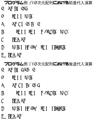
プログラム例

1: CRS

方式における前進代入演算

1. do i = 1, n

2.

tmp = w(i)

3.

do j = lrowptr(i), lrowptr(i + 1)

− 1

4.

tmp = tmp

− lval(j) ∗ w(lcolind(j))

5.

end do

6.

w(i) = omega

∗ tmp ∗ pivot(i)

7. end do

プログラム例

2

に

CRS

方式を使用した場合の後退代入演算

のプログラム例を示す．

uval

は上三角行列

U

の非零要素

の配列，

urowptr

は上三角行列

U

のポインタ配列，

ucolind

は上三角行列

U

のインデックス配列である．

プログラム例

2: CRS

方式における後退代入演算

1. do i = n, 1,

−1

2.

tmp = w(i)

3.

do j = urowptr(i), urowptr(i + 1)

− 1

4.

tmp = tmp

− uval(j) ∗ w(ucolind(j))

5.

end do

6.

u(i) = omega

∗ tmp ∗ pivot(i)

7. end do

プログラム例

1

，同例

2

のように，密行列を

CRS

方式で格

納する場合，

4

行目の

w(ucolind(j))

において間接参照が

行われる．まず，

ucolind(j)

で配列

w

の番地を参照してか

ら，

w

に格納されている値を参照する．

w

の値を求めるた

めに

2

個の配列を参照するため，計算時間が長くなる．

3.2

密行列専用の格納方法と前進後退代入演算

密行列用に行列要素を

2

次元配列で格納する

[6]

．

2

次元

配列では全ての行列要素を格納する．プログラム例

3

，同

例

4

に

2

次元配列における前進後退代入のプログラム例を

示す

[3]

．

mat

は行列要素を格納した

2

次元配列である．

プログラム例

3: 2

次元配列における前進代入演算

1. do i = 1, n

2.

tmp = w(i)

3.

do j = 1, i

− 1

4.

tmp = tmp

− mat(j, i) ∗ w(j)

5.

end do

6.

w(i) = omega

∗ tmp ∗ pivot(i)

7. end do

プログラム例

4: 2

次元配列における後退代入演算

1. do i = n, 1,

−1

2.

tmp = w(i)

3.

do j = i + 1, n

4.

tmp = tmp

− mat(j, i) ∗ w(j)

5.

end do

6.

w(i) = omega

∗ tmp ∗ pivot(i)

7. end do

プログラム例

3

，同例

4

のように，行列要素を

2

次元配列

で格納した場合，

4

行目の配列

w

の値を直接参照で求めら

れるため，密行列に対して反復法の高速化が期待できるが，

どの程度改善できるかを知りたい．

4.

数値実験

4.1

電磁界解析で現れたテスト行列

同志社大学理工学部 藤原・高橋研究室より提供された

電磁界解析モデルのテスト行列に対する密行列専用版反

復法の収束性を調査する．使用した行列は

2

個で，共に

密行列である．行列

boxshield (

次元数：

4,902)

は

2

個の

コイルに挟まれた箱の解析モデル，行列

problem13 (

次元

数：

16,800)

は

TEAM (Testing Electromagnetic Analysis

Method) Workshop

により公開されている検証用の解析モ

デルである．図

1

に行列

boxshield

，

図

2

に行列

problem13

の解析モデルとメッシュ図と磁束密度分布を示す．ここ

で，メッシュ図は対称性から図

1

では全体の

1/8

，図

2

で

は

1/4

のみ表示した．

4.1.1

計算機環境と計算条件

計算機は

Dell PowerEdge R210

（戦略名：

Sandy Bridge,

CPU

：

Intel Xeon E3-1220

，クロック周波数：

3.1GHz

，メ

モリ：

8.2Gbytes

，

L3

キャッシュメモリ：

8.2Mbytes, OS

：

Red Hat Linux Enterprise

）を使用した．プログラムは

For-tran90

を用いて実装し，コンパイラは

Intel Fortran

Com-piler ver.12.1.3

を使用した．最適化オプションは

“-O3”

を

使用した．右辺項は物理的条件から得られる値を用いた．収

束判定条件は相対残差の

2

ノルム：

||r

||2/

||r0||2

≤ 10

とした．初期近似解

x

はすべて

0

とした．前処理は対

角スケーリングと

E-SSOR

前処理を使用した．最大反

図

1

boxshield

Fig. 1

Analytic model, mesh and distribution of density

in case of matrix boxshield.

図

2

problem13

Fig. 2

Analytic model, mesh and distribution of density

in case of matrix problem13.

復回数は

10000

回とした．解法は

GPBiCG

法

[14]

，

GP-BiCG variant4

法

(

以下，

GPBiCG v4

と表記

)[1]

，

BiCGSafe

法

[10]

，

GMRES

法

[12]

，

GBiCGSTAB(s,L)[13]

法の

5

種

類を使用した．

4.1.2

実験結果

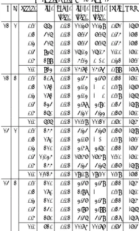
表

1

，表

2

に行列

boxshield

に対する

E-SSOR

前処理つ

き反復法の収束性を示す．表中の

GMRES

法のリスタート

係数は

500

，加速係数は

0.1

から

1.0

まで

0.1

刻みで実験を

行った．ここで，

0.6

から

0.9

までの実験結果については全

ての解法で最短で収束するケースが無かったので，省略し

た．

GBiCGStab(s,L)

法では

s

を

4,8,10,12,14

，

L

を

1,2

と

変化させた．

TRR

は

True Relative Residual

の略で常用

対数

log

(

||b − Ax

||2

/

||b − Ax0||2

)

の値を意味する．

“acc-c.”

は

accelerated coefficient

の略で加速係数を示す．

また，

“pre-t.”

は前処理にかかった時間，

“itr-t.”

は反復計

表

1

boxshield

E-SSOR

Table 1

Convergence rate of four E-SSOR preconditioned

it-erative methods for matrix boxshield.

method acc-c. itr. pre-t. itr-t. tot-t. ratio TRR [sec.] [sec.] [sec.]

GPBiCG 0.1 125 0.02 4.20 4.22 0.26 -8.0 0.2 180 0.02 6.03 6.05 0.38 -8.0 0.3 150 0.02 5.02 5.05 0.31 -7.6 0.4 205 0.02 6.85 6.87 0.43 -8.5 0.5 230 0.02 7.68 7.70 0.48 -8.2 1.0 480 0.02 16.01 16.04 1.00 -8.0 GPBiCG v4 0.1 105 0.02 3.54 3.56 0.22 -8.5 0.2 215 0.02 7.19 7.21 0.45 -8.5 0.3 260 0.02 8.69 8.71 0.54 -8.1 0.4 170 0.02 5.69 5.71 0.36 -8.1 0.5 195 0.02 6.54 6.56 0.41 -8.3 1.0 620 0.02 20.68 20.71 1.29 -8.4 BiCGSafe 0.1 235 0.02 7.86 7.88 0.49 -8.7 0.2 225 0.02 7.52 7.54 0.47 -8.0 0.3 230 0.02 7.69 7.71 0.48 -8.2 0.4 170 0.02 5.69 5.71 0.36 -8.7 0.5 185 0.02 6.18 6.21 0.39 -8.1 1.0 720 0.02 23.99 24.01 1.50 -8.1 GMRES 0.1 142 0.02 2.34 2.37 0.15 -8.2 0.2 137 0.02 2.25 2.27 0.14 -8.2 0.3 145 0.02 2.39 2.41 0.15 -8.1 0.4 156 0.02 2.58 2.60 0.16 -8.0 0.5 174 0.02 2.87 2.89 0.18 -7.9 1.0 390 0.02 6.61 6.63 0.41 -7.5

間である．

ratio

は

GPBiCG

法の加速係数

1.0

における合

計時間を

1

としたときの他の解法の合計時間の比である．

表

1,

表

2

より以下のことがわかる．

( 1 ) GMRES

法で加速係数が

0.2

のとき，合計時間は

2.27

秒で最も速く収束した．

( 2 )

次いで，

GPBiCGStab

法が

(s,L)=(10,2)

で加速係数

0.2

のとき

2.97

秒で収束した．

表

3,

表

4

に行列

problem13

に対する

E-SSOR

前処理

つき反復法の収束性を示す．

表

3

，表

4

より以下のことがわかる．

( 1 ) GMRES

法で加速係数が

0.3

のとき，合計時間は

43.02

秒で最も速く収束した．

( 2 )

次いで，

BiCGSafe

法が加速係数

0.2

のとき

88.83

秒で

収束した．

4.2

積分方程式法によるテスト行列の場合

積分法試験法による解析で得られた解析モデルの行列

2

個で，次元数

11,308

，非零要素数

127,870,864(

小規模モデ

ル

)

と次元数

20,756

，非零要素数

430,811,536(

中規模モデ

ル

)

でどちらも密行列である．

4.2.1

計算機環境と計算条件

計算はすべて倍精度浮動小数点演算で行った．小規模モ

デルに対しては，計算機は

Dell PowerEdge R210

（戦略

名：

Sandy Bridge, CPU

：

Intel Xeon E3-1220

，クロック

表

2

boxshield

E-SSOR

GBiCGStab(s,L)

Table 2

Convergence rate of E-SSOR preconditioned

GBiCGStab(s,L) method for matrix boxshield.

(a) in case of s = 4

∼ 10

s L acc-c. itr. pre-t. itr-t. tot-t. ratio TRR [sec.] [sec.] [sec.]

4 1 0.1 max 0.02 - - - 60.9 0.2 225 0.02 4.30 4.32 0.27 -8.1 0.3 3,010 0.02 57.42 57.44 3.58 -8.1 0.4 1,575 0.02 30.02 30.04 1.87 -8.0 0.5 510 0.02 9.74 9.76 0.61 -8.0 1.0 1,060 0.02 20.23 20.25 1.26 -7.2 4 2 0.1 190 0.02 3.33 3.36 0.21 -6.9 0.2 180 0.02 3.16 3.18 0.20 -7.8 0.3 210 0.02 3.68 3.71 0.23 -7.9 0.4 240 0.02 4.22 4.25 0.27 -7.9 0.5 260 0.02 4.56 4.58 0.29 -7.8 1.0 800 0.02 13.98 14.00 0.87 -8.1 8 1 0.1 792 0.02 14.04 14.06 0.88 -5.6 0.2 243 0.02 4.32 4.34 0.27 -7.1 0.3 1,719 0.02 30.44 30.46 1.90 -8.0 0.4 1,035 0.02 18.31 18.33 1.14 -7.5 0.5 720 0.02 12.76 12.79 0.80 -7.3 1.0 945 0.02 16.74 16.76 1.05 -7.1 8 2 0.1 198 0.02 3.35 3.37 0.21 -7.4 0.2 180 0.02 3.05 3.07 0.19 -7.0 0.3 198 0.02 3.35 3.37 0.21 -7.7 0.4 216 0.02 3.65 3.68 0.23 -7.1 0.5 270 0.02 4.56 4.58 0.29 -7.2 1.0 684 0.02 11.52 11.54 0.72 -7.4 10 1 0.1 209 0.02 3.65 3.68 0.23 -7.0 0.2 297 0.02 5.19 5.21 0.33 -7.0 0.3 187 0.02 3.28 3.30 0.21 -7.5 0.4 528 0.02 9.20 9.22 0.58 -7.4 0.5 1,507 0.02 26.21 26.23 1.64 -7.5 1.0 1,111 0.02 19.34 19.36 1.21 -7.7 10 2 0.1 198 0.02 3.31 3.33 0.21 -6.8 0.2 176 0.02 2.95 2.97 0.19 -6.8 0.3 198 0.02 3.32 3.34 0.21 -6.7 0.4 220 0.02 3.69 3.71 0.23 -7.3 0.5 286 0.02 4.78 4.81 0.30 -6.6 1.0 682 0.02 11.39 11.41 0.71 -7.2

周波数：

3.1GHz

，メモリ：

8.2Gbytes

，

L3

キャッシュメモ

リ：

8.2Mbytes

，

OS

：

Red Hat Linux Enterprise

）を使用

した．プログラムは

Fortran90

を用いて実装し，コンパイ

ラは

Intel Fortran Compiler ver.12.1.3

を使用した．中規

模モデルに対しては，計算機は

CX400

（

CPU

：

Intel Xeon

E5-2690

，クロック周波数：

2.7GHz

，メモリ：

128Gbytes

，

キャッシュメモリ：

20Gbytes

，

OS

：

Red Hat Linux

Enter-prise

）を使用した．プログラムは

Fortran90

を用いて実装

し，コンパイラは

Fujitsu Fortran Compiler

を使用した．

最適化オプションは

“-O3”

を使用した．右辺項は物理的

条件から得られる値を用いた．収束判定条件は相対残差の

2

ノルム：

||r

||2/

||r0||2

≤ 10

とした．初期近似解

x

(b) in case of s = 12 and 14

s L acc-c. itr. pre-t. itr-t. tot-t. ratio TRR [sec.] [sec.] [sec.]

12 1 0.1 663 0.02 11.37 11.39 0.71 -6.7 0.2 416 0.02 7.14 7.16 0.45 -7.2 0.3 416 0.02 7.14 7.16 0.45 -7.2 0.4 936 0.02 16.03 16.05 1.00 -7.0 0.5 299 0.02 5.13 5.15 0.32 -7.1 1.0 923 0.02 15.82 15.84 0.99 -7.8 12 2 0.1 208 0.02 3.45 3.47 0.22 -7.0 0.2 182 0.02 3.03 3.05 0.19 -6.7 0.3 182 0.02 3.03 3.05 0.19 -6.6 0.4 234 0.02 3.88 3.90 0.24 -6.9 0.5 260 0.02 4.31 4.33 0.27 -7.0 1.0 676 0.02 11.19 11.21 0.70 -6.5 14 1 0.1 255 0.02 4.34 4.37 0.27 -6.9 0.2 180 0.02 3.07 3.10 0.19 -7.1 0.3 210 0.02 3.58 3.60 0.22 -7.4 0.4 1,035 0.02 17.57 17.59 1.10 -7.0 0.5 255 0.02 4.34 4.36 0.27 -6.9 1.0 1,125 0.02 19.09 19.11 1.19 -7.2 14 2 0.1 210 0.02 3.47 3.49 0.22 -6.5 0.2 180 0.02 2.98 3.00 0.19 -6.0 0.3 210 0.02 3.47 3.49 0.22 -6.5 0.4 240 0.02 3.97 3.99 0.25 -6.6 0.5 270 0.02 4.46 4.49 0.28 -6.8 1.0 720 0.02 11.85 11.87 0.74 -7.4 表

3

problem13

E-SSOR

Table 3

Convergence rate of four E-SSOR preconditioned

it-erative methods for matrix problem13.

method acc-c. itr. pre-t. itr-t. tot-t. ratio TRR [sec.] [sec.] [sec.]

GPBiCG 0.1 330 1.49 128.73 130.22 0.35 -7.9 0.2 275 0.25 106.49 106.74 0.28 -6.5 0.3 385 0.33 149.55 149.87 0.40 -8.3 0.4 300 0.25 116.41 116.67 0.31 -8.2 0.5 320 0.25 124.10 124.35 0.33 -8.2 1.0 975 0.25 377.05 377.30 1.00 -8.0 GPBiCG v4 0.1 350 0.25 135.56 135.81 0.36 -8.0 0.2 295 0.26 114.52 114.77 0.30 -8.3 0.3 245 0.25 95.04 95.29 0.25 -8.1 0.4 265 0.25 102.86 103.12 0.27 -8.5 0.5 295 0.25 114.57 114.83 0.30 -8.3 1.0 675 0.26 262.53 262.79 0.70 -8.1 BiCGSafe 0.1 305 0.25 118.11 118.36 0.31 -8.4 0.2 230 0.25 88.58 88.83 0.24 -7.7 0.3 230 0.25 89.22 89.47 0.24 -8.4 0.4 250 0.25 97.90 98.15 0.26 -8.2 0.5 270 0.25 104.16 104.42 0.28 -8.3 1.0 915 0.25 359.08 359.33 0.95 -8.0 GMRES 0.1 229 0.25 43.32 43.57 0.12 -8.0 0.2 230 0.25 43.55 43.81 0.12 -8.0 0.3 229 0.25 42.76 43.02 0.11 -8.2 0.4 241 0.25 45.00 45.25 0.12 -8.1 0.5 258 0.25 48.25 48.50 0.13 -7.9 1.0 594 0.25 112.21 112.46 0.30 -7.6

前処理を使用した．最大反復回数は

10000

回とした．

4

problem13

E-SSOR

GBiCGStab(s,L)

Table 4

Convergence rate of E-SSOR preconditioned

GBiCGStab(s,L) method for matrix problem13.

(a) in case of s = 4

∼ 10

s L acc-c. itr. pre-t. itr-t. tot-t. ratio TRR [sec.] [sec.] [sec.]

4 1 0.1 max 0.320 - - - 31.6 0.2 max 0.683 - - - 46.2 0.3 1,125 0.697 249.11 249.80 0.66 -7.4 0.4 550 1.222 122.22 123.44 0.33 -7.6 0.5 790 0.440 174.94 175.38 0.46 -8.0 1.0 1,795 0.626 398.33 398.96 1.06 -7.9 4 2 0.1 350 0.356 71.03 71.39 0.19 -6.5 0.2 370 0.402 75.13 75.53 0.20 -7.5 0.3 390 0.605 80.49 81.10 0.21 -7.6 0.4 400 0.876 81.42 82.29 0.22 -6.8 0.5 470 0.663 95.54 96.20 0.25 -8.1 1.0 1,270 0.388 257.88 258.27 0.68 -7.1 8 1 0.1 max 0.967 - - - 16.3 0.2 468 0.644 96.14 96.78 0.26 -6.8 0.3 450 0.528 92.67 93.20 0.25 -6.7 0.4 378 1.554 78.16 79.71 0.21 -6.9 0.5 837 0.780 172.48 173.26 0.46 -7.1 1.0 1,260 0.386 258.63 259.01 0.69 -6.3 8 2 0.1 324 0.494 63.81 64.30 0.17 -5.6 0.2 324 0.411 64.08 64.49 0.17 -6.1 0.3 360 0.455 71.59 72.04 0.19 -5.9 0.4 324 0.405 63.50 63.90 0.17 -7.1 0.5 414 0.510 80.56 81.07 0.21 -6.7 1.0 1,152 0.413 225.67 226.08 0.60 -6.5 10 1 0.1 341 0.448 68.84 69.29 0.18 -6.6 0.2 528 0.521 106.53 107.05 0.28 -6.6 0.3 330 0.731 66.65 67.38 0.18 -6.6 0.4 440 0.337 88.89 89.23 0.24 -6.9 0.5 506 0.316 102.15 102.47 0.27 -6.7 1.0 1,507 0.476 303.83 304.31 0.81 -6.8 10 2 0.1 308 0.424 59.56 59.98 0.16 -5.4 0.2 330 0.635 63.97 64.60 0.17 -6.2 0.3 308 0.485 60.68 61.17 0.16 -6.0 0.4 352 0.455 69.69 70.14 0.19 -6.4 0.5 396 0.323 76.36 76.68 0.20 -6.6 1.0 990 0.331 190.70 191.03 0.51 -6.7

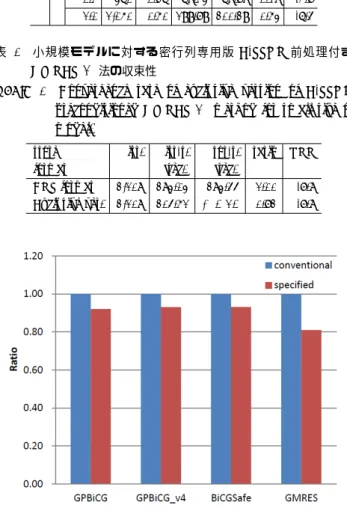
4.2.2

実験結果

表

5

に小規模モデルに対する密行列専用版

E-SSOR

前

処理付き

GMRES(k)

法の収束性を示す．リスタート係数

は

2200

，加速係数は

0.7

で実験を行った．

表

5

より密行列専用版

E-SSOR

前処理

GMRES(k)

法が

従来法より

18%

計算時間が短縮された

.

表

6

に中規模モデルに対する密行列専用版

E-SSOR

前

処理付き反復法の収束性を示す．ここで，加速係数は

0.6

から

1.0

まで

0.1

刻みで変化させた．表中の

ratio

は従来版

の合計時間を

1

とした時の専用版の合計時間の比である．

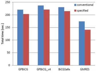
図

3

に各解法の従来版と専用版の合計時間比を示す．

図

4

に各解法の従来版と専用版の合計時間を比較した図

を示す．

(b) in case of s=12 and 14

s L acc-c. itr. pre-t. itr-t. tot-t. ratio TRR [sec.] [sec.] [sec.]

12 1 0.1 481 0.53 95.58 96.10 0.25 -6.3 0.2 299 0.79 59.59 60.38 0.16 -6.0 0.3 312 0.82 62.16 62.98 0.17 -6.5 0.4 351 0.55 69.79 70.34 0.19 -6.4 0.5 559 0.58 111.10 111.68 0.30 -7.3 1.0 1,625 0.41 321.51 321.91 0.85 -7.2 12 2 0.1 286 0.46 54.88 55.34 0.15 -5.2 0.2 286 0.34 54.90 55.24 0.15 -5.4 0.3 338 0.56 64.80 65.36 0.17 -6.1 0.4 338 0.51 64.82 65.33 0.17 -6.3 0.5 364 0.53 70.24 70.77 0.19 -6.3 1.0 1,014 0.37 194.14 194.51 0.52 -6.5 14 1 0.1 330 0.50 65.02 65.52 0.17 -6.9 0.2 330 0.45 65.14 65.59 0.17 -6.3 0.3 315 0.48 62.15 62.62 0.17 -6.5 0.4 375 0.26 75.18 75.44 0.20 -6.7 0.5 585 0.26 114.77 115.03 0.30 -5.0 1.0 1,395 0.26 273.53 273.79 0.73 -6.5 14 2 0.1 300 0.57 57.29 57.86 0.15 -5.5 0.2 300 0.34 57.19 57.53 0.15 -5.0 0.3 330 0.26 62.79 63.04 0.17 -4.8 0.4 360 0.26 68.52 68.77 0.18 -4.7 0.5 360 0.26 68.53 68.78 0.18 -5.7 1.0 1,050 0.50 199.79 200.29 0.53 -6.4 表

5

E-SSOR

GMRES(k)

Table 5

Convergence rate of exclusive version of E-SSOR

preconditioned GMRES(k) method for small size of

model.

store itr. itr-t. tot-t. ratio TRR format [sec.] [sec.]

CRS format 2,108 283.03 283.44 1.00 -7.8 Exclusive ver. 2,108 204.51 204.64 0.72 -7.8

図

3

Fig. 3

Comparison of the conventional CRS version and

exclu-sive version of iterative methods in view of the ratio of

total computation time.

表

6

E-SSOR

Table 6

Convergence rate of exclusive version of four E-SSOR

preconditioned iterative methods for middle size of

model.

method acc-c. itr. pre-t. itr-t. tot-t. ratio TRR [sec.] [sec.] [sec.]

GPBiCG 0.6 180 1.82 225.14 226.96 1.00 -8.2 (CRS) 0.7 175 1.81 218.87 220.68 1.00 -8.0 0.8 175 1.78 218.96 220.74 1.00 -8.1 0.9 195 1.81 243.91 245.72 1.00 -8.7 1.0 180 1.81 225.02 226.83 1.00 -8.3 GPBiCG 0.6 180 0.43 208.57 209.01 0.92 -8.2 (exclu.) 0.7 175 0.43 202.76 203.20 0.92 -8.0 0.8 175 0.44 202.77 203.20 0.92 -8.1 0.9 195 0.44 225.83 226.28 0.92 -8.7 1.0 180 0.44 208.54 208.97 0.92 -8.3 GPBiCG v4 0.6 180 1.81 223.19 224.99 1.00 -8.2 (CRS) 0.7 190 1.78 235.47 237.25 1.00 -8.0 0.8 185 1.79 229.26 231.05 1.00 -8.3 0.9 175 1.81 216.84 218.65 1.00 -8.1 1.0 185 1.81 229.44 231.25 1.00 -8.1 GPBiCG v4 0.6 180 0.44 209.07 209.51 0.93 -8.2 (exclu.) 0.7 190 0.43 220.61 221.05 0.93 -8.0 0.8 185 0.44 214.82 215.26 0.93 -8.3 0.9 175 0.43 203.39 203.82 0.93 -8.1 1.0 185 0.44 214.82 215.25 0.93 -8.1 BiCGSafe 0.6 180 1.81 222.59 224.41 1.00 -8.0 (CRS) 0.7 185 1.80 228.67 230.47 1.00 -8.2 0.8 175 1.79 216.31 218.10 1.00 -8.1 0.9 185 1.80 228.80 230.60 1.00 -8.2 1.0 195 1.81 241.01 242.82 1.00 -8.2 BiCGSafe 0.6 180 0.44 208.59 209.02 0.93 -8.0 (exclu.) 0.7 185 0.45 214.29 214.74 0.93 -8.2 0.8 175 0.44 202.76 203.20 0.93 -8.1 0.9 185 0.44 214.38 214.82 0.93 -8.2 1.0 195 0.44 225.97 226.40 0.93 -8.2 GMRES 0.6 261 2.84 177.50 180.33 1.00 -8.1 (CRS) 0.7 252 2.84 171.37 174.22 1.00 -8.0 0.8 257 2.83 174.32 177.16 1.00 -7.9 0.9 263 2.84 178.73 181.57 1.00 -7.9 1.0 278 2.84 188.58 191.41 1.00 -7.8 GMRES 0.6 261 0.44 145.78 146.22 0.81 -8.1 (exclu.) 0.7 252 0.44 140.66 141.11 0.81 -8.0 0.8 257 0.44 143.39 143.84 0.81 -7.9 0.9 263 0.44 146.70 147.14 0.81 -7.9 1.0 278 0.45 155.12 155.57 0.81 -7.8

表

6

，図

3

，図

4

より以下のことがわかる．

( 1 )

全ての解法で従来版よりも専用版のほうが計算速度が

向上した．

( 2 )

特に，

GMRES

法では専用版が従来版と比べて

19%

計

算時間が短縮された．

( 3 )

同様に，

GPBiCG

法では専用版が従来版より

7.9%

短

縮された

.

5.

まとめ

本論文では，密行列に対して行列要素を

2

次元配列で

図

4

Fig. 4

Comparison of the conventional CRS version and

exclu-sive version of iterative methods in view of total

com-putation time.

全ての要素を格納する，密行列専用の

E-SSOR

前処理付

き反復法の高速化の度合いを調査した．数値実験では，密

行列専用版

E-SSOR

前処理つきの

GMRES

法が最も速く

収束した．中規模モデルに対して

GMRES

法では密行列

専用版の合計時間が従来版より

19%

短縮された．一方で，

GPBiCG

法では

7.9%

短縮された．以上より，

GMRES

法

が最も高速化され，密行列に対して有効であることが示さ

れた．

参考文献

[1]

Abe, K., Sleijpen, Gerard L.G.: Solving linear equations

with a stabilized GPBiCG method, Appl. Numer. Math.,

doi:10.1016/j.apnum.2011.06.10, 2011.

[2]

Axelsson, O. : A generalized SSOR method, BIT, Vol.12,

pp.443-467, 1972.

[3]

Barrett, R., Berry, M., et al.: Templates for the Solution

of Linear Systems: Building Blocks for Iterative

Meth-ods,

長谷川里美，長谷川秀彦，藤野清次：反復法

Templates

，

朝倉書店，

1996

．

[4]

Benzi, M.: Preconditioning Techniques for Large Linear

Systems: A Survey, Journal of computational Physics,

Vol.182, pp.418-477, 2002.

[5]

Chan, T. F., van der Vorst, H. A.: Approximate and

In-complete Factorizations, Parallel Numerical Algorithms,

ICASE/LaRC Interdisciplinary Series in Sci. and Eng.,

Kluwer Academic, Vol.4, pp.167-202, 1997.

[6]

Chen, K: Matrix Preconditioning Techniques and

Appli-cations, Cambridge Monographs on Applied and

Com-putational Mathematics, 2005.

[7]

Chen, K.: On a class of preconditioning methods for

dense linear systems from boundary elements, SIAM J.

Sci. Comput., Vol.20, No.2, pp.684-698, 1998.

[8]

Chen, X., Toh, K. C., Phoon, K. K.: A modified SSOR

preconditioner for sparse symmetric indefinite linear

sys-tems of equations, Int. J. Numer. Meth. Engng, Vol.65,

pp.785-807, 2006.

[9]

Eisenstat, S. C.:

Efficient implementation of a class

of preconditioned conjugate gradient methods, SIAM J.

Sci. Stat. Compute., Vol.2, pp.1-4, 1981.

[10]

Fujino, S., Fujiwara, M., Yoshida, M.: A proposal of

preconditioned BiCGSafe method with safe convergence,

Proc. of The 17th IMACSWorld Congress on

Scien-tific Computation, Appl. Math. Simul., CD-ROM, Paris,

France, 2005.

[11]

村上啓一，藤野清次

:

残余行列の活用による

Eisenstat

版

前処理付き

IDR(s)-R2

法の並列化，研究室セミナー資料，

2.2011.

[12]

Saad, Y. : Iterative Methods for Sparse Linear Systems

2nd edition, SIAM, Philadelphia, 2003.

[13]

塚田健，深堀康紀，谷尾真明，杉原正顕

:

自動残差修正機

能付き

GBiCGSTAB(s,L)

法，数理解析研究所講究録，第

1733

巻，

pp.149-159, 2011.

[14]

Zhang, S.-L. :

GPBi-CG: Generalized product-type

methods preconditionings based on Bi-CG for solving

nonsymmetric linear systems, SIAM J. Sci. Comput.,

pp.537-551, 1997.