PAPER
Approximation and Analysis of Non-linear Equations in a
Moment Vector Space
Hideki SATOH†a), Member
SUMMARY Moment vector equations (MVEs) are pre-sented for use in approximating and analyzing multi-dimensional non-linear discrete- and continuous-time equations. A non-linear equation is expanded into simultaneous equations of generalized moments and then reduced to an MVE of a coefficient matrix and a moment vector. The MVE can be used to analyze the sta-tistical properties, such as the mean, variance, covariance, and power spectrum, of the non-linear equation. Moreover, we can approximately express a combination of non-linear equations by using a combination of MVEs of the equations. Evaluation of the statistical properties of Lorenz equations and of a combina-tion of logistic equacombina-tions based on the MVE approach showed that MVEs can be used to approximate non-linear equations in statistical measurements.
key words: approximation, linearization, non-linear, statistics 1. Introduction
Many everyday systems are large, complicated, and non-linear. They often comprise a large number of small systems that interact in a complicated manner. To design and control these systems, we need to know their various properties. However, even if we knew all the properties of the elements that constitute the tar-get system, we cannot always control the elements. We may find it more useful to know the macroscopic and statistical properties of the target system, such as the moments, response time, and power spectra, than the microscopic and minute ones.
Various methods have been developed for approx-imately analyzing non-linear systems, including the Galerkin method and ones based on perturbation anal-ysis and asymptotic analanal-ysis. These methods expand the solution into a series and determine the coefficient of each function. By using these methods, we can ob-tain approximate solutions to deterministic differential equations [1], [2], [3], stochastic differential equations [4], and partial differential equations of a probability density function [5]. A linearization approach that cre-ates a linear model by linearizing the target system at the equilibrium point is widely used. With this model, we can use linear control theory [6] to control the target system.
However, approximate solutions obtained by the
Manuscript received June 6, 2005.
Final manuscript received October 3, 2005.
†The author is with the Future University-Hakodate,
Hakodate-shi, 041-8655 Japan. a) E-mail: [email protected]
above methods are rather complex, or the linear model obtained in the neighborhood of the equilibrium point is too simple to express global properties. Thus, we can-not always use these methods to control everyday sys-tems or to investigate their macroscopic and statistical properties. Moment vector equations (MVEs), which were recently developed [7], can be used to analyze the statistical properties, such as the mean, variance, covariance, and power spectrum, for one-dimensional discrete-time systems. However, this does not mean that MVEs always approximate the non-linear systems or that we can use MVEs as an approximation of non-linear systems to control them. Moreover, MVEs should also work for multi-dimensional or continuous-time systems.
The systematic procedures presented in this paper solve these problems by expanding a previous work on one-dimensional discrete-time systems [7]. Using these procedures, we can construct MVEs and use them to analyze the statistical properties of multi-dimensional non-linear discrete- and continuous-time equations. A combination of non-linear equations can be expressed approximately by using a combination of MVEs of the non-linear equations, demonstrating that an MVE ap-proximates a non-linear system itself. Evaluation of the statistical properties of Lorenz equations and those of a combination of logistic equations by using MVEs showed that MVEs can be used as an approximation of non-linear equations in statistical measurements. 2. MVEs for Multi-dimensional Systems This section presents systematic procedures by expand-ing a previous work [7] to approximate various non-linear equations to MVEs.
2.1 MVEs for Discrete-time Systems
Let us consider the following multi-dimensional discrete-time non-linear systems
s`(n + 1) = f`(s(n)) for 1 ≤ ` ≤ L, (1)
where s def= t(s
1,· · ·,sL), L is the number of variables,
n = 0, 1, 2, · · · is a discrete time, S def= {s|ˇs` ≤ s` ≤
ˇ
s`+ T` for 1 ≤ ` ≤ L} is the domain of the definition
Let {φi} be a linear independent system that
con-stitutes the basis of S (see Appendix A), and let us abbreviate the variables defined above as follows:
s`def= s`(n), s0 ` def = s`(n + 1), sdef= s(n), (2) φidef= φi(s(n)), φ0 i def = φi(s(n + 1)).
To derive an MVE, let us assume the following with respect to Eq. (1):
Assumption 1: We can expand E[φ0
i|s] in a Fourier series as follows: E[φ0 i|s] = N X j=0 aijφj+ εi(s), (3)
where E[·] is a mathematical expectation, εi(s) is a
residual, and φ0 is a constant. By using Eq. (3), we can expand E[φ0
i] as follows: E[φ0 i] = Z φ0 ip(φ0i)dφ0i = Z φ0i Z p(s)p(φ0i|s)dsdφ0i = Z p(s)E[φ0i|s]ds = N X j=0 aijE[φj] + E[εi(s)], (4)
where p(·) denotes a probability density function. When {φi} is an orthonormal basis, aij is obtained by
using Eq. (A· 2) as follows:
aij=
Z
Sφi(f (s))φj(s)ds, (5)
where f def= t(f
1, · · · , fL). Let us assume that
E[εi(s)] = 0, and let us define ˜x(n) and ˜A as follows:
˜
x(n)def= t(E[φ0(s(n))], · · · , E[φN(s(n))]),
˜ Adef= a00 · · · a0N .. . . .. ... aN 0· · · aN N .
Then Eq. (4) is expressed by the following MVE: ˜
x(n + 1) = ˜A˜x(n). (6) In Assumption 1, we assumed that E[φ0(s(n))] is con-stant φ0. Thus, by rewriting Eq. (6), we obtain an MVE, which is a linear equation in a moment vector space, as follows:
x(n + 1) = Ax(n) + B, (7) where A, B, and x(n) are defined as follows:
x(n)def= t(E[φ 1(s(n))], · · · , E[φN(s(n))]), Adef= a11 · · · a1N .. . . .. ... aN 1· · · aN N , Bdef= a10φ0 .. . aN 0φ0 .
2.2 MVEs for Continuous-time Systems
In this section, MVEs for multi-dimensional continuous-time non-linear systems are derived in the same manner as in Sect. 2.1. Let us consider the following systems
˙s`(t) = f`(s(t)) for 1 ≤ ` ≤ L, (8)
where t is a continuous time, ˙s`(t) denotes ds`(t)/dt,
and s(t) ∈ S.
Because E[·] is a linear operator, dE[φi(s(t))]/dt
= E[dφi(s(t))/dt]. Thus, by using the following
abbre-viation instead of Eq. (2)
s`def= s`(t), s0 ` def = ds`/dt, sdef= s(t), (9) φidef= φi(s(t)), φ0 i def = dφi(s(t))/dt,
and assuming that Assumption 1 holds, we can obtain the following equation from Eq. (4):
dE[φi]/dt = E[φ0i] = N X j=0 aijE[φj] + E[εi(s)]. (10)
Here, by using Eq. (8), we can express φ0
i as follows: φ0 i= L X `=1 ∂φi ∂s` f`(s).
Thus, when {φi} is an orthonormal basis, aij is
ob-tained by using Eq. (A· 2) as follows:
aij = Z S( L X `=1 ∂φi(s) ∂s` f`(s))φj(s)ds. (11)
Let us assume that E[εi(s)] = 0, and let us define ˜x(t)
by ˜
x(t)def= t(E[φ
0(s(t))], · · · , E[φN(s(t))]).
From Eq. (10), we obtain the following MVE:
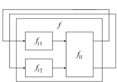
Fig. 1 A combination of three discrete-time systems.
where ˙˜x(t)def= d˜x(t)/dt. As in Sect. 2.1, we assume that E[φ0(s(t))] is constant φ0. Thus, the above equation can be rewritten as the following MVE:
˙x(t) = Ax(t) + B, (13)
where ˙x(t)def= dx(t)/dt, and x(t) is defined by
x(t)def= t(E[φ1(s(t))], · · · , E[φN(s(t))]).
2.3 A Combination of Discrete-time Systems
Let us consider the following three discrete-time sys-tems in order to explain how we can express a combi-nation of discrete-time systems:
sI`(n + 1) = fI`(sI`(n)) for ` = 1, 2,
sII(n + 1) = fII(sII(n)).
By using bases {φi} and {φ`i}, we can express the
MVEs of fI1, fI2, and fII by ˜ xI`(n + 1) = ˜AI`x˜I`(n) for ` = 1, 2, ˜ xII(n + 1) = ˜AIIx˜II(n), where ˜
xI`(n)def= t(E[φ`0(sI`(n))], · · · , E[φ`N`(sI`(n))]), ˜
xII(n)def= t(E[φ0(sII(n))], · · · , E[φN(sII(n))]), ˜ φdef= t(φ 0, · · · , φN), ˜ φ` def = t(φ `0, · · · , φ`N`).
Let us now construct a new system, f , by connecting the above three systems, fI1, fI2, and fII, as shown in Fig. 1. That is,
s(n + 1) = f (s(n)), s(n + 1)def= sII(n + 1), s(n)def= t(ts I1(n),tsI2(n)), f def= fII(fI1, fI2). (14)
For given ˜φ`, let ˜φ and ˜x(n) be
˜
x(n)def= t(E[φ
0(s(n))], · · · , E[φN(s(n))]),
˜
φdef= ˜φ1⊗ ˜φ2, (15) and let us express the MVE of f by
˜
x(n + 1) = ˜A˜x(n), (16) where ⊗ denotes a matrix direct product. From Eqs. (14) and (15), the following equation holds:
˜
x(n) = ˜xI1(n) ⊗ ˜xI2(n). (17) Because fI1and fI2 are independent, by using the fol-lowing new variables
˜ x0I1def= ˜AI1x˜I1(n), ˜ x0I2 def = ˜AI2x˜I2(n),
the input to fII can be expressed by ˜x0I1⊗ ˜x0I2. There-fore, by using the following formulae with respect to the matrix direct product [9]
t(A ⊗ B) =tA ⊗tB, (18)
(A ⊗ C)(B ⊗ D) = (AB) ⊗ (CD), (19)
we obtain the following equation: ˜
x(n + 1) = ˜AII(˜x0I1⊗ ˜x0I2) = ˜AII( ˜AI1⊗ ˜AI2)˜x(n).
Therefore, coefficient matrix ˜A in the MVE of f is
expressed by the combination of coefficient matrices in the MVEs of fI1, fI2, and fII as follows:
˜
A = ˜AII( ˜AI1⊗ ˜AI2). (20) Because it is assumed that E[φ0(s(n))] is constant φ0, Eq. (16) can be rewritten as Eq. (7) in the same manner as Eq. (6).
3. Analysis
Let λi be the ith eigenvalue of matrix A in the MVE
of Eq. (7) or (13), ei be the eigenvector for λi, Λ def=
diag[λ1, · · · , λN], and M def= [e1, · · · , eN]. In this
sec-tion, various statistical properties of non-linear equa-tions are derived based on A, Λ, and M by expanding a previous work [7]. To evaluate in Sect. 4 the accuracy of the statistical properties that are obtained based on MVEs, the properties based on a numerical solution of non-linear equations are also defined in this section. 3.1 Moments for Discrete Time Systems
In this section, moments of s`(n) in Eq. (1) are derived
under the following assumption:
Assumption 2: Equation (7), which is an MVE of Eq. (1), has a unique equilibrium point, and it does not diverge. That is, ∀λi6= 1, and ∀|λi| ≤ 1 [8].
3.1.1 Moments Based on a Numerical Solution From the time average of the sequence of s`(n), s`(n +
1), · · · obtained from the numerical solution of Eq. (1), moment hhs`(n)kii and covariance hhs`(n)sν(n)ii
based on a numerical solution are computed, where hh·ii denotes a finite-time average, and it is defined for a discrete-time variable x(n) as follows:
hhx(n)iidef= 1
τmax τmaxX−1
τ =0
x(n + τ ). (21)
Variance σ`2and correlation coefficient ρ`νare obtained
by the following equations:
σ2
` = hhs`(n)2ii − hhs`(n)ii2, (22)
ρ`ν= hhs`(n)sν(n)ii − hhs`(n)iihhsν(n)ii
σ`σv
. (23)
3.1.2 Moments Based on an MVE
Let infinite-time average hx(n)i of discrete-time vari-able x(n) be [10]
hx(n)idef= lim
τmax→∞ 1 τmax τmaxX−1 τ =0 x(n + τ ). (24)
From Appendix B.1, ¯xdef= lim
n→∞hx(n)i
† is equal to x∗
in Eq. (7), where x∗is the equilibrium point of x(n) in
Eq. (7). Thus, when Assumption 2 holds, (I − A)−1
exists, and ¯x is derived by the following equation [8]:
¯
x = x∗
= (I − A)−1B, (25)
where I is a unit matrix.
Let us now expand E[s`(n + 1)] and E[s`(n +
1)sν(n + 1)] in a Fourier series as follows in the same
manner as in Eq. (4): E[s`(n + 1)] = E[f`(s(n))] = N X j=0 ζ`;jE[φj(s(n))], (26) E[s`(n + 1)sν(n + 1)] = E[f`(s(n))fν(s(n))] = N X j=0 ζ`ν;jE[φj(s(n))]. (27)
At the equilibrium point of Eq. (7), E[φi(s(n +
1))] = E[φi(s(n))], and thus, Eqs. (26) and (27) yield
E[s`(n + 1)] = E[s`(n)] and E[s`(n + 1)sν(n + 1)] = †The reason we have to consider lim
n→∞hx(n)i is explained
in Appendix B.
E[s`(n)sν(n)]. Let these values be E∗[φi(s)], E∗[s`],
and E∗[s
`sν], respectively. From Eqs. (25) through
(27), moment E[sk `] def = lim n→∞hE[s`(n) k]i for k = 1, 2
and covariance E[s`sν] def= lim
n→∞hE[s`(n)sν(n)]i based
on the MVE of Eq. (7) are computed by using the fol-lowing equations: E[s `] = E∗[s`] = N X j=0 ζ`;jE∗[φj(s)], (28) E[s`sν] = E∗[s`sν] = N X j=0 ζ`ν;jE∗[φj(s)]. (29) Here, E∗[φ
j(s)] is an element of x∗. The variance and
correlation coefficient are obtained in the same manner as in Eqs. (22) and (23).
3.2 Power Spectra for Discrete-time Systems
Periodogram [10], which is defined based on a finite-duration Fourier transform and is an estimation of the power spectrum, of s`(n) in Eq. (1) is derived in this
section, assuming that Assumption 2 holds.
3.2.1 A Periodogram Based on a Numerical Solution Let F`(k) be the time average of the Fourier transform
of sequence s`(n), s`(n + 1), · · · obtained from the
nu-merical solution of Eq. (1) as follows:
F`(k)def= hh W −1X m=0
s`(n + m)e−ıω0mkii, (30)
where ı is an imaginary unit, k ∈ {0, 1, · · · , W − 1}, and ω0def= 2π/W . From the above equation, we obtain periodogram S``(k) based on the numerical solution of
Eq. (1) as follows:
S``(k)def= 1
W|F`(k)|
2. (31)
3.2.2 A Periodogram Based on an MVE
Correlation function r`ν(m) of s`(n) and sν(n) is
de-fined by
r`ν(m)def= lim
n→∞hE[s`(n)sν(n + m)]i. (32)
The right-hand side of Eq. (32) is derived from Eq. (35) described in Section 3.2.3. From Eq. (32), the power spectrum of s`(n) based on the MVE of Eq. (1), ˆS``(k),
ˆ
S`ν(k) = W −1X m=0
r`ν(m)e−ıω0mk. (33)
For ν 6= `, the above equation denotes the cross power spectrum of s`(n) and sν(n) [10].
3.2.3 The MVE of the Correlation Function
The right-hand side of Eq. (32) is derived in this section. Consider the following simultaneous equations of Eqs. (7) and (26): E[sν(n + 1)] E[φ1(s(n + 1))] .. . E[φN(s(n + 1))] = ˆAν E[sν(n)] E[φ1(s(n))] .. . E[φN(s(n))] + ˆBν, where ˆ Aνdef= 0 ζν;1 · · · ζν;N 0 a11 · · · a1N .. . ... . .. ... 0 aN 1 · · · aN N , ˆBν def = ζν;0φ0 a10φ0 .. . aN 0φ0 . Let ˆx`ν(m; n) be ˆ x`ν(m; n)def= E[s`(n)sν(n + m)] E[s`(n)φ1(n + m)] .. . E[s`(n)φN(n + m)] .
By replacing g`(s(n)) with s`(n) in Eq. (A· 13) in
Ap-pendix C, we obtain the following equation: ˆ
x`ν(m + 1; n) = ˆAνxˆ`ν(m; n) + E[s`(n)] ˆBν. (34)
To eliminate the effect of the initial value of Eq. (1) and to derive the power spectrum even when Eq. (34) oscillates †, consider ¯ˆx
`ν(m) def= lim
n→∞hˆx`ν(m; n)i. We
obtain ¯ˆx`ν(m) from the limit of the time average of Eq.
(34) for n → ∞ as follows:
¯ˆx`ν(m + 1) = ˆAν¯ˆx`ν(m) + E∗[s`] ˆBν. (35)
By computing the above equation for m = 0, 1, 2, · · · step by step, we can obtain the right-hand side of Eq. (32). The initial value of the above equation, ¯ˆx`ν(0), is
derived in Appendix D.1.
3.3 Moments for Continuous-time Systems
This section shows the moments of s`(t) in Eq. (8) in
the same manner as in Sect. 3.1 under the following assumpiton:
Assumption 3: Equation (13), which is an MVE of Eq. (8), has a unique equilibrium point, and it does not diverge. That is, ∀λi6= 0, and ∀Re[λi] ≤ 0 [8].
3.3.1 Moments Based on a Numerical Solution Moment hhs`(t)kii and covariance hhs`(t)sν(t)ii are
de-rived based on a numerical solution by solving Eq. (8) numerically. Here, hh·ii is a finite time average, and it is defined for continuous variable x(t) as follows:
hhx(t)iidef= 1
τmax Z τmax
0
x(t + τ )dτ . (36) The variance and correlation coefficient are derived in the same manner as in Eqs. (22) and (23).
3.3.2 Moments Based on an MVE
Let hx(t)i be the infinite-time average of continuous variable x(t) as follows:
hx(t)idef= lim
τmax→∞ 1 τmax Z τmax 0 x(t + τ )dτ . (37)
Appendix B.2 shows that ¯xdef= lim
n→∞hx(t)i is equal to
equilibrium point x∗ in Eq. (13). Thus, if Assumption
3 holds, A−1 exists [8], and ¯x is expressed by
¯
x = x∗
= −A−1B. (38)
Let us expand E[s`(t)] and E[s`(t)sν(t)] as follows:
E[s`(t)] = N X j=0 η`;jE[φj(s(t))], (39) E[s`(t)sν(t)] = N X j=0 η`ν;jE[φj(s(t))]. (40)
Because E[φi(s)] is a constant at the equilibrium point,
Eqs. (39) and (40) show that E[s`(t)] and E[s`(t)sν(t)]
are also constants at the equilibrium point. Let each constant be E∗[φ
i(s)], E∗[s`], and E∗[s`sν],
respec-tively. From Eqs. (38) through (40), moment E[sk `]
def = lim
t→∞hE[s`(t)
k]i for k = 1, 2 and covariance E[s `sν] def=
lim
t→∞hE[s`(t)sν(t)]i are obtained based on the MVE of
Eq. (13) by using the following equations:
E[s `] = E∗[s`] = N X j=0 η`;jE∗[φj(s)], (41) E[s `sν] = E∗[s`sν] = N X j=0 η`ν;jE∗[φj(s)]. (42) Here, E∗[φ
j(s)] is an element of x∗. The variance and
correlation coefficient are obtained in the same manner as in Eqs. (22) and (23).
3.4 Power Spectra for Continuous-time Systems The power spectrum of s`(t) in Eq. (8) is derived in
this section, assuming that Assumption 3 holds. 3.4.1 A Periodogram Based on a Numerical Solution Let s`(0), s`(∆t), s`(2∆t), · · · be a sequence obtained
by solving Eq. (8) numerically and sampling solution
s`(t) at periodic intervals ∆t. By rewriting s`(n∆t)
as s`(n) and applying s`(n) to Eqs. (30) and (31), we
can derive periodogram S``(k), as an estimation of the
power spectrum of s`(t) based on a numerical solution.
3.4.2 A Periodogram Based on an MVE
Correlation function r`ν(τ ) of s`(t) and sν(t) is defined
by the following equation:
r`ν(τ )def= lim
t→∞hE[s`(t)sν(t + τ )]i. (43)
The right-hand side of the above equation is derived from Eq. (47) in Sect. 3.4.3. Let r`ν(0), r`ν(∆t),
r`ν(2∆t), · · · be a sequence obtained by sampling r`ν(τ )
at periodic intervals ∆t. Let us rewrite r`ν(m∆t) as
r`ν(m) and apply r`ν(m) to Eq. (33). Then we obtain
periodgram ˆS``(k) based on an MVE††.
3.4.3 The MVE of the Correlation Function
The right-hand side of Eq. (43) is derived in this section. First, let us expand E[s`(t)sν(t + τ )] by using Eq. (39)
as follows: E[s`(t)sν(t+τ )] = E[s`(t) N X j=0 ην;jφj(s(t + τ ))] = ην;0φ0E[s`(t)] + N X j=1 ην;jE[s`(t)φj(s(t + τ ))] = ην;0φ0E[s`(t)]+ N X j=1 ην;jxˆ`(τ ; t), (44) where ˆ x`(τ ; t)def= E[s`(t)φ1(s(t + τ ))] .. . E[s`(t)φN(s(t + τ ))] .
Next, let us derive ˆx`(τ ; t). From the linearity of
E[·], the following equation holds:
††Although we can obtain the power spectrum by
deriv-ing the Fourier transform of Eq. (43) analytically, sequence
r`ν(m) obtained by sampling r`ν(τ ) is used here because of
the restriction in computing time.
dE[s`(t)φi(s(t + τ ))]/dτ = E[s`(t)dφi(s(t + τ ))/dτ ].
Thus, we obtain the following equation for τ ≥ 0 by replacing g`(s(t + τ )) with s`(t) in Eq. (A· 13) in
Ap-pendix C:
dˆx`(τ ; t)/dτ = Aˆx`(τ ; t) + E[s`(t)]B.
By solving the above equation, we obtain the following equation [8]:
ˆ
x`(τ ; t) = M diag[eλiτ]M−1xˆ`(0; t)
+M diag[λ−1
i (eλiτ−1)]M−1E[s`(t)]B. (45)
Let us consider the time average of the above equa-tion at the limit as t tends to ∞†. Then we obtain the
following equation:
¯ˆx`(τ ) = M diag[eλiτ]M−1¯ˆx`(0)
+M diag[λ−1
i (eλiτ−1)]M−1E∗[s`]B, (46)
where ¯ˆx`(τ ) def= lim
t→∞hˆx`(τ ; t)i. By replacing
lim
t→∞hE[s`(t)sν(t + τ )]i with r`ν(τ ), limt→∞hˆx`(τ ; t)i with
¯ˆx`(τ ), and lim
t→∞hE[s`(t)]i with E ∗[s
`] in the time
av-erage of Eq. (44) for t → ∞, we obtain correlation function r`ν(τ ) as follows: r`ν(τ ) = ην;0φ0E∗[s`] + N X j=1 ην;j¯ˆx`(τ ). (47)
Initial value ¯ˆx`(0) of the above equation is derived in
Appendix D.2.
4. Performance Evaluation
To evaluate the accuracy of the MVEs for continuous-time systems described in Eq. (13), the statistical prop-erties, such as the mean, standard deviation, and peri-odogram, of each variable in the following Lorenz equa-tions [11] were investigated:
˙s1 = α1(−s1+ s2),
˙s2 = s1(α2− s3) − s2, (48) ˙s3 = s1s2− α3s3,
where (α1, α2, α3) = (10, 28, 8/3). The attractor is shown in Fig. 2. Figures 3 through 6 show the statistical properties of Lorenz equations derived based on MVEs (see Sects. 3.3.2 and 3.4.2) for various values of N`,
where N`for ` = 1, 2, 3 denotes the degree of the Fourier
series (see Appendix A), (ˇs1, ˇs2, ˇs3) = (−25, −25, 0), (T1, T2, T3) = (50, 50, 50), and W = 512. To evaluate the accuracy of the statistical properites derived based on the MVE, those based on the numerical solution of Eq. (48) (see Sects. 3.3.1 and 3.4.1) are also shown in these figures (indicated ”Num.” on the abscissa axis).
From these figures, the mean, standard deviation, and periodogram based on the MVE approach to those
Fig. 2 Lorenz attractor.
Fig. 3 Mean and standard deviation of Lorenz equations.
based on the numerical solutions as N`increases. If
As-sumption 1 holds, that is, the Fourier series converges as
N` increases, the statistical properties converge to the
true values as N` increases. We can also see the
differ-ence between the stochastic motions in s1 and s2 and the deterministic motion in s3 from the periodograms. Thus, an MVE can contain statistical properties, such as the mean, standard deviation, and periodogram, of a non-linear equation.
Although we can derive the statistical properties of a non-linear equation based on an MVE, this does not mean that the MVE always approximates the non-linear equation itself. To show that MVEs can be an approximation of non-linear equations, the statistical properties of a combination of the following logistic equations [11] were evaluated by using a combination of their MVEs:
sI`(n + 1) = fI`(sI`(n)) def
= α`sI`(n)(1 − sI`(n)) for ` = 1, 2, where α1 = 3.8 and α2 = 3.9. Consider the following discrete-time non-linear system:
s(n + 1) = f (s(n)), (49)
Fig. 4 Periodograms of Lorenz equations (s1 ).
Fig. 5 Periodograms of Lorenz equations (s2 ).
Fig. 6 Periodograms of Lorenz equations (s3 ).
which is constructed by connecting the above two lo-gistic equations as shown in Eq. (14) and Fig. 1, where
Fig. 7 Moments and correlation coefficient of a combination of logistic equations. sII(n + 1) = fII(sII(n)) = CsII(n), Cdef= · 1 − c c c 1 − c ¸ .
That is, s1(n) and s2(n) are independent when c = 0, and s1(n) and s2(n) affect each other when c 6= 0.
Based on Sects. 3.1.2 and 3.2.2, the statistical properties, such as the means, standard deviations, cor-relation coefficients, and periodograms, of s1(n) and
s2(n) in Eq. (49) were evaluated using MVEs, which are constructed as shown in Sect. 2.3 from the MVEs of
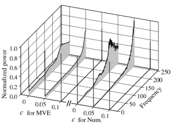
fI1, fI2, and fII. The statistical properties are shown in Figs. 7 through 9 (labeled ”MVE” on the abscissa axis), where W = 512, T`= 1, ˇs`= 0, and N`= 16 for
` = 1, 2. The periodograms for c = 0 were multiplied by
3, those for c = 0.05 were multiplied by 2, and those for
c = 0.1 were divided by 40 in order to arrange them in
the same figures. To evaluate the accuracy of the MVE approach, the statistical properties derived based on the numerical solution of Eq. (49) were also evaluated according to Sects. 3.1.1 and 3.2.1, and they are shown in each figure (labeled ”Num.” on the abscissa axis).
As shown in the figures, the change in c was re-flected both in the statistical properties obtained based on MVEs and in those obtained based on numerical so-lutions. That is, the means and standard deviations became equal, the correlation coefficients changed from 0 to −1, and the periodograms became line spectra, when the value of c changed from 0 to 0.1. These results show that the statistical properties of a combination of non-linear equations are expressed by using a combina-tion of MVEs of these non-linear equacombina-tions. Therefore, we can conclude that MVEs are an approximation of non-linear equations in statistical measurements. 5. Conclusion
Moment vector equations (MVEs) can be used to
ap-Fig. 8 Power spectrum of a combination of logistic equations (s1).
Fig. 9 Power spectrum of a combination of logistic equations (s2).
proximate and analyze non-linear equations. We can not only analyze the statistical properties, such as the mean, variance, covariance, and power spectrum, of non-linear equations based on MVEs but also express a combination of non-linear equations by using a com-bination of MVEs of these equations. Evaluation of the statistical properties of Lorenz equations and those of a combination of logistic equations showed that we can analyze the statistical properties of these equations based on MVEs and that we can use MVEs as an ap-proximation of multi-dimensional non-linear discrete-and continuous-time equations in statistical measure-ments. Because MVEs can be used to approximate non-linear systems and MVEs are linear, it is expect that we can easily perform stability analysis and con-trol various non-linear systems. I will report on these items in the near future.
Appendix A: The Basis of MVEs
The Fourier series expansion of function g(s) with re-spect to sdef= t(s 1, · · · , sL) ∈ S is defined by [12] g(s) = X k∈Z h(k)K(s, k), (A· 1) h(k)def= Z Sg(s)K(s, k)ds, (A· 2) where k def= t(k 1, · · · , kL), Z def= {k|0 ≤ k` ≤
N` for 1 ≤ ` ≤ L}, h(k)s are Fourier coefficients,
and {K(s, k)} is an orthogonal basis defined by the product of one dimensional orthogonal basis K`(s`, k`)
as follows: K(s, k)def= L Y `=1 K`(s`, k`). (A· 3)
Let φi(s) be the basis of the MVE defined by
φi(s)def= K(s, k), (A· 4)
where the relationship between i and k ∈ Z is obtained by the following equation:
i = L X `=1 k` L Y ν=`+1 Nν. (A· 5)
Dimension N of Matrix A is obtained as follows:
N =
L
Y
`=1
(N`+ 1) − 1.
Let L(s, k) be an orthonormal basis for s ∈ [ˇs, ˇs + T ] defined by [12]: L(s, k) = r 2k + 1 T P (2 s − ˇs T − 1, k), (A· 6)
where P (x, k) is the Legendre polynomial for x ∈ [−1, 1] defined by P (x, 0) = 1, P (x, 1) = x, P (x, 2) = (3x2− 1)/2, P (x, 3) = (5x3− 3x)/2, .. . .
In Sect. 4, K`(s`, k`) is set to L(s`, k`) for ∀`.
Appendix B: The Average of the Moment
Vector
Under Assumptions 2 and 3, although Eqs. (7) and (13) have a unique equilibrium point and do not diverge,
the moment vector often oscillates. To derive moments from the equilibrium point even when the moment vec-tor oscillates and to eliminate the effect of the initial value of the moment vector, the relationship between the time average of the moment vector and the equilib-rium point is derived in this section.
B.1 The Average for Discrete-time Systems
Let x∗ be the equilibrium point of x(n) in Eq. (7).
When Assumption 2 holds, ∀λi 6= 1, and (I − A)−1
exists. Thus, we obtain x∗ as follows [8]:
x∗= (I − A)−1B.
The solution of x(n) is expressed by [8]
x(n) = M ΛnM−1(x(0) − x∗) + x∗. (A· 7) From the above equation and Assumption 2, time av-erage ¯x is obtained as follows:
¯ x def= lim n→∞hx(n)i = M ( lim n→∞hΛ ni)M−1(x(0) − x∗) + x∗ = x∗. (A· 8)
B.2 The Average for Continuous-time Systems Let x∗ be the equilibrium point of x(t) in Eq. (13).
When Assumption 3 holds, A−1 exists, and x∗ is
ex-pressed by the following equation [8]:
x∗= −A−1B. (A· 9)
The solution to Eq. (13) is as follows [8]:
x(t) = M diag[eλit]M−1x
0 +M diag[λ−1
i (eλit− 1)]M−1B. (A· 10)
By using Eqs. (A· 9) and (A· 10), we obtain time aver-age ¯x as follows: ¯ x def= lim t→∞hx(t)i = lim t,τmax→∞ 1 τmax(M diag[ Z eλi(t+τ )dτ ]M−1x 0 +M diag[ Z 1 λie λi(t+τ )dτ − Z 1 λidτ ]M −1B) = −M diag[λ−1i ]M−1B = −A−1B = x∗. (A· 11)
Appendix C: The MVE of the Correlation
Function
to vector variable s. For convenience, let us use the fol-lowing abbreviations both for continuous- and discrete-time systems: sdef= s(n) or s(t + τ ), hidef= hi(s(n)) or hi(s(t + τ )), h0 i def = hi(s(n + 1)) or dhi(s(t + τ ))/dτ, g`def= g`(s(n)) or g`(s(t + τ )).
In this section, correlation function E[g`h0i] is derived.
When Assumption 1 holds, we obtain the following equation both for continuous- and discrete-time sys-tems: E[h0i|s] = N X j=0 aijhj+ εi(s). (A· 12)
Note that h0is a constant. Assuming that E[εi(s)] = 0
in Eq. (A· 12), we can expand E[g`h0i] as follows:
E[g`h0i] = Z Z g`h0ip(h0i, s)dh0ids = Z g` Z h0 ip(h0i|s)dh0ip(s)ds = Z g`E[h0i|s]p(s)ds = Z g`( N X j=0 aijhj)p(s)ds = N X j=1 aijE[g`hj] + ai0h0E[g`].
Therefore, using coefficient matrix A, the MVE of cor-relation function E[g`h0i] is expressed as follows:
E[g`h01] .. . E[g`h0N] = A E[g`h1] .. . E[g`hN] + E[g`] a10h0 .. . aN 0h0 .(A· 13)
Appendix D: The Initial Value of the Correla-tion FuncCorrela-tion
Initial values of Eqs. (35) and (47) are derived in this section.
D.1 Discrete-time Systems
We obtain the following equation by expanding
E[s`(n + 1)φi(s(n + 1))] in a series with respect to
E[φj(s(n))] as follows: E[s`(n + 1)φi(s(n + 1))] = E[f`(s(n))φi(f (s(n)))] = N X j=0 ξ`;ijE[φj(s(n))].
By using the above equation, Eq. (29), and ˜x(n) defined
in Sect. 2.1, ˆx`ν(0; n + 1) can be expressed by
ˆ x`ν(0; n + 1) = ˆΞ`νx(n),˜ (A· 14) where ˆΞ`ν is defined by ˆ Ξ`νdef= ζ`ν;0 ζ`ν;1 · · · ζ`ν;N ξ`;10 ξ`;11 · · · ξ`;1N .. . ... . .. ... ξ`;N 0 ξ`;N 1 · · · ξ`;N N .
Here, ζ`ν;j is a coefficient used in Eq. (29). Let ˜x∗ be
the equilibrium point of ˜x(n). Because lim
n→∞h˜x(n)i =
˜
x∗ holds from Appendix B.1, we obtain the initial val-ues of Eq. (35), ¯ˆx`ν(0), by the following equation:
¯ˆx`ν(0) = ˆΞ`νx˜∗. (A· 15)
D.2 Continuous-time Systems
By expanding E[s`(t)φi(s(t))] in a Fourier series with
respect to E[φj(s(t))], we obtain
E[s`(t)φi(s(t))] = N X j=0 ξ`;ijE[φj(s(t))]. Thus, ˆx`(0; t) is obtained by ˆ x`(0; t) = Ξ`x(t),˜
where ˜x(t)def= t(E[φ
0(s(t))], · · · , E[φN(s(t))]) and Ξ`def= ξ`;10 ξ`;11 · · · ξ`;1N .. . ... . .. ... ξ`;N 0 ξ`;N 1 · · · ξ`;N N . (A· 16) Let ˜x∗ def= t(φ
0,tx∗) and ¯˜x(t) def= lim
t→∞h˜x(t)i. From
Appendix B.2, ¯˜x(t) = ˜x∗. Therefore, we can obtain the initial values of Eq. (47), ¯ˆx`(0), by the following
equation:
¯ˆx`(0) = Ξ`x˜∗.
References
[1] L. Azrar, R. Benamar, and R. G. White, “A semi-analytical approach to the non-linear dynamic response problem of S-S and C-C beams at large vibration amplitudes. Part I. General theory and application to the single mode approach to free and forced vibration analysis,” J. Sound Vib., vol. 224, no. 2, pp. 183–207, July 1999.
[2] A. F. Vakakis and M. E. King, “Resonant oscillations of a weakly coupled nonlinear layered system,” Acta Mech., vol. 128, no. 1-2, pp. 59-80, 1998.
[3] K. Komatsu and H. Takata, “A Formal Linearization by the Chebyshev Interpolation and Its Applications”, Pro-ceedings of the IEEE Conference on Decision and Control, Vol.1 of 4, pp.70–75, 1996.
[4] R. V. Bobryk, “Stochastic equations of the Langevin type under a weakly dependent perturbation,” J. Stat. Phys., vol. 70, no. 3/4, pp. 1045–1056, Feb. 1993.
[5] G. Muscolino, G. Ricciardi, and M. Vasta, “Stationary and non-stationary probability density function for non-linear oscillators,” Int. J. Non-Linear Mech., vol. 32, no. 6, pp. 1051–64, Nov. 1997.
[6] K. J. Astrom, Introduction to Stochastic Control Theory, Academic Press, 1970.
[7] H. Satoh, “A Statistical Analysis of Non-linear Equations based on a Linear Combination of Generalized Moments,” IEICE Tans. Fundamentals, vol. E87-A, no. 12, pp. 3381– 3388, Dec. 2004.
[8] D. G. Luenberger, Introduction to Dynamic Systems The-ory Models & Applications, John Wiley & Sons, New York, 1979.
[9] R. Bellman, Introduction to Matrix Analysis, McGRAW-HILL, New York, 1960.
[10] A. V. Oppenheim and R. W. Schafer, Digital Signal Pro-cessing, Prentice-Hall, London, 1975.
[11] E. Ott, Chaos in Dynamical Systems Second edition, Cam-bridge, UK, 2002.
[12] I. N. Bronshtein and K. A. Semendyayev, Handbook of Mathematics, Springer-Verlag, 1985.