Golden optimal path in discrete-time dynamic
optimization processes
Seiichi IWAMOTO and Masami YASUDA
Department of Economic Engineering
Graduate School of Economics, Kyushu University
Fukuoka 812-8581, Japan
tel&fax. +81(92)642-2488, email: [email protected]
and
Department of Mathematical Science
Faculty of Science, Chiba University
Chiba 263-8522, Japan
tel&fax. +81(43)290-3662, email: [email protected]
Abstract
We are concerned with dynamic optimization processes from a viewpoint of Golden optimality. A path is called Golden if any state moves to the next state repeating the same Golden section in each transition. A policy is called Golden if it, together with a relevant dynamics, yields a Golden path. The probelm is whether an optimal path/policy is Golden or not. This paper minimizes a quadratic criterion and maximizes a square-root criterion over an infinite horizon. We show that a Golden path is optimal in both optimizations. The Golden optimal path is obtained by solving a corresponding Bellman equation for dynamic programming. This in turn admits a Golden optimal policy.
1
Introduction
Recently the Golden optimal solution, its duality, and its equivalence have been discussed in static optimization problems [4–6]. In this paper we consider the Golden optimal solution in dynamic optimization problems.
We consider two typical types of criterion — quadratic and square-root — in a deter-ministic optimization. We minimize quadratic criteria
I(x) = ∞ X n=0 £ x2 n+ (xn− xn+1)2 ¤ , J(x) = ∞ X n=0 £ (xn− xn+1)2+ x2n+1 ¤
and maximize square-root criteria K(x) = ∞ X n=0 βn¡√x n + √ xn− xn+1 ¢ , L(x) = ∞ X n=0 βn¡√x n− xn+1 + √ xn+1 ¢
, respectively. Here β is 0 < β < 1. The differences between I and J and between K and L are J(x) = I(x) − x2 0 L(x) = K(x) + ∞ X n=0 ¡ βn−1− βn¢ √xn (β−1 = 0).
We show that a Golden path is optimal in these four optimization problems. The Golden optimal path is obtained by solving Bellman equation for dynamic programming [3, 7].
2
Golden Paths
A real number φ = 1 + √ 5 2 ≈ 1.618is called Golden number [1,2,8]. It is the larger of the two solutions to quadratic equation
x2− x − 1 = 0. (1)
Sometimes (1) is called Fibonacci quadratic equation. The Fibonacci quadratic equation has two real solutions: φ and its conjugate φ := 1 − φ. We note that
φ + φ = 1, φ · φ = −1. Further we have
φ2 = 1 + φ, φ2 = 2 − φ
φ2 + φ2 = 3, φ2· φ2 = 1.
A point (2 − φ)x splits an interval [0, x] into two intervals [0, (2− φ)x] and [(2 − φ)x, x]. A point (φ − 1)x splits the interval into [0, (φ − 1)x] and [(φ − 1)x, x]. In either case, the length constitutes the Golden ratio (2 − φ) : (φ − 1) = 1 : φ. Thus both divisions are the Golden section.
Definition 2.1 A sequence x : {0, 1, . . .} → R1 is called Golden if and only if either
xt+1
xt
= φ − 1 or xt+1 xt
= 2 − φ. Lemma 2.1 A Golden sequence x is either
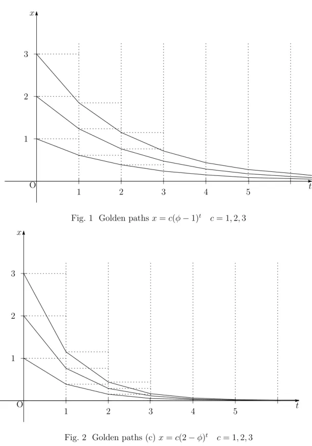
O x t + + + + + + + + + + 2 1 3 4 5 1 2 3
Fig. 1 Golden paths x = c(φ − 1)t c = 1, 2, 3
O x t + + + + + + + + + + 2 1 3 4 5 1 2 3
We remark that
(φ − 1)t= φ−t, (2 − φ)t = (1 + φ)−t
where
φ − 1 = φ−1 ≈ 0.618, 2 − φ = (1 + φ)−1 ≈ 0.382
Let us introduce a controlled linear dynamics with real parameter b as follows.
xt+1 = bxt+ ut t = 0, 1, . . . (2)
where u : {0, 1, . . .} → R1is called control. If u
t = pxt, the control u is called proportional,
where p is a real constant, proportional rate. A sequence x satisfying (2) is called path. Definition 2.2 A proportional control u on dynamics (2) is called Golden if and only if it generates a Golden path x.
Lemma 2.2 A proportional control ut= pxt on (2) is Golden if and only if
p = −b + φ − 1 or p = −b + 2 − φ. (3)
3
Control processes
This section minimizes two quadratic cost functions
∞ X n=0 £ x2 n+ (xn− xn+1)2 ¤ and ∞ X n=0 £ (xn− xn+1)2+ x2n+1 ¤ . Both problems are solved as a control process with criterion
∞ X n=0 ¡ x2 n+ u2n ¢ and ∞ X n=0 ¡ u2 n+ x2n+1 ¢
under a common additive dynamics with a given initial state xn+1 = bxn+ un, x0 = c
where c ∈ R1.
3.1
Quadratic in current state
Let us now consider a control process with an additive transition T (x, u) = bx + u. Here b is a constant, which represents a characteristics of the process :
minimize ∞ X n=0 ¡ x2 n+ u2n ¢ subject to (i) xn+1= bxn+ un C(c) n ≥ 0 (ii) − ∞ < un< ∞ (iii) x0 = c.
Let v(c) be the minimum value of C(c). Then the value function v satisfies Bellman equation [3]: v(x) = min −∞<u<∞ £ x2+ u2+ v(bx + u)¤. (4)
Eq. (4) has a quadratic form v(x) = vx2, where v ∈ R1.
Lemma 3.1 The control process C(c) with characteristic value b (∈ R1) has a
propor-tional optimal policy f∞, f (x) = px, and a quadratic minimum value function v(x) = vx2,
where v = b2+ √ b4+ 4 2 , p = − v 1 + v b.
The proportional optimal policy f∞ splits at any time an interval [0, x] into [0, (b +
p)x] = · 0, bx 1 + v ¸ and · bx 1 + v , x ¸
. In particular, when b = 1, the quadratic coefficient v is reduced to the Golden number
φ = 1 + √
5
2 ≈ 1.618 Further the division of [0, x] into
· 0, x 1 + φ ¸ and · x 1 + φ, x ¸ is Golden. A quadratic function w(x) = ax2 is called Golden if a = φ.
Theorem 3.1 The control process C(c) with characteristic value b = 1 has a Golden optimal policy f∞, f (x) = (1 − φ)x, and the Golden quadratic minimum value function
v(x) = φx2.
3.2
Qquadratic in next state
Here we consider the cost function r : X×U → R1 which is quadratic in current control
and next state :
r(x, u) = u2+ (bx + u)2.
Then a control process is represented by the following sequential minimization problem : minimize ∞ X n=0 ¡ u2n+ x2n+1¢ subject to (i) xn+1= bxn+ un C0(c) n ≥ 0 (ii) − ∞ < un< ∞ (iii) x0 = c.
The value function v satisfies Bellman equation [3]:
v(x) = min
−∞<u<∞
£
u2+ (bx + u)2+ v(bx + u)¤. (5)
Lemma 3.2 The control process C0(c) with characteristic value b has a proportional
op-timal policy f∞, f (x) = px, and a quadratic minimum value function v(x) = vx2, where
v = b2− 2 + √ b4 + 4 2 , p = − 1 + v 2 + vb. The policy f∞ splits an interval [0, x] into
· 0, bx 2 + v ¸ and · bx 2 + v, x ¸ . When b = 1, the coefficient v is reduced to the inverse Golden number
φ−1 = φ − 1 = −1 + √
5
2 ≈ 0.618
Further the division of [0, x] into [0, (2 − φ)x] and [(2 − φ)x, x] is Golden. A quadratic function w(x) = ax2 is called inverse Golden if a = φ−1.
Theorem 3.2 The control process C0(c) with characteristic value b = 1 has a Golden
optimal policy f∞, f (x) = (1 − φ)x, and the inverse Golden quadratic minimum value
function v(x) = (φ − 1)x2.
4
Allocation processes
This section maximizes two discounted square-root reward functions
∞ X n=0 βn¡√xn + √ xn− xn+1 ¢ and ∞ X n=0 βn¡√xn− xn+1 + √ xn+1 ¢ . Both problems are solved as an allocation process with criterion
∞ X n=0 βn(√xn + √ un) and ∞ X n=0 βn(√un +√xn+1)
under a common subtractive dynamics with a given initial state xn+1 = xn− un, x0 = c
where c ≥ 0.
4.1
Square-root in current state
Let us now consider an allocation process with a subtractive transition T (x, u) = x − u : Maximize ∞ X n=0 βn(√x n + √ un) subject to (i) xn+1= xn− un A(c) n ≥ 0 (ii) 0 ≤ un≤ xn (iii) x0 = c.
Let v(c) be the maximum value of A(c). Then the maximum value function v satisfies the following Bellman equation:
v(x) = Max
0≤u≤x
£√
x +√u + βv(x − u)¤. (6)
Eq. (6) has a square-root form v(x) = v√x , where v ∈ R1.
Let us adopt a proportional policy f∞ (f (x) = px) with proportional rate p (0 <
p < 1). Then state x under the control u = px goes deterministically to the next state T (x, u) = x − u = x − px = (1 − p)x. Thus we have x = (1 − p)x + px. The state transition of control process A(c) governed by the proportional policy f∞ means that the current
control u = px splits the state interval [0, x] into two intervals [0, (1−p)x] and [(1−p)x, x]. When the split yields a Golden section, the proportional policy f∞ (f (x) = px) is called
Golden.
Lemma 4.1 The allocation process A(c) has a proportional optimal policy f∞, f (x) = px,
and a square-root maximum value function v(x) = v√x , where
v = 2
1 − β2 , p =
(1 − β2)2
(1 + β2)2 .
We remark that the coefficient v is the solution to v = 1 +p1 + (βv)2, v ≥ 2.
Let us solve 1 − p = φ − 1 or 2 − φ. Then we have the following result.
Theorem 4.1 When β = φ (1 −√φ − 1 ) ≈ 0.346 or β = √φ −√φ − 1 ≈ 0.486, the proportional policy f∞, f (x) = px, is Golden optimal.
4.2
Square-root in next state
Now we consider an allocation process with transition T (x, u) = x − u : Maximize ∞ X n=0 βn(√u n +√xn+1) subject to (i) xn+1 = xn− un A0(c) n ≥ 0 (ii) 0 ≤ un ≤ xn (iii) x0 = c.
Let v(c) be the maximum value of A0(c). Then the maximum value function v satisfies
an optimality equation:
v(x) = Max
0≤u≤x
£√
u +√x − u + βv(x − u)¤. (7)
Eq. (7) has a square-root solution v(x) = v√x , where v ∈ R1.
Let us adopt a proportional policy f∞ (f (x) = px) with p (0 < p < 1). Then the
Lemma 4.2 The allocation process A0(c) has a proportional optimal policy f∞, f (x) =
px, and a square-root maximum value function v(x) = v√x , where
v = β + p 2 − β2 1 − β2 , p = 1 − βp2 − β2 2 .
Note that the coefficient v is the positive solution to v = p1 + (1 + βv)2.
By solving 1 − p = φ − 1, we have the following result.
Theorem 4.2 When β = p1 − 2√2φ − 3 ≈ 0.168, the proportional policy f∞, f (x) =
px, is Golden optimal.
References
[1] A. Beutelspacher and B. Petri, Der Goldene Schnitt 2., ¨uberarbeitete und erweiterte Auflange, ELSEVIER GmbH, Spectrum Akademischer Verlag, Heidelberg, 1996. [2] R.A. Dunlap, The Golden Ratio and Fibonacci Numbers, World Scientific Publishing
Co.Pte.Ltd., 1977.
[3] S. Iwamoto, Theory of Dynamic Program: Japanese, Kyushu Univ. Press, Fukuoka, 1987.
[4] S. Iwamoto, Cross dual on the Golden optimum solutions, Mathematical Economics, Research Institute for Mathematical Sciences, Kyoto University, RIM S K ˆokyˆuroku 1443, 2005, pp. 27–43.
[5] S. Iwamoto, The Golden optimum solution in quadratic programming, Ed. W. Taka-hashi and T. Tanaka, Proceedings of the International Conference on Nonlinear Anal-ysis and Convex AnalAnal-ysis (Okinawa, 2005), Yokohama Publishers, Yokohama, 2006, pp.1–7.
[6] S. Iwamoto, The Golden trinity — optimility, inequality, identity —, Mathemat-ical Economics, Research Institute for MathematMathemat-ical Sciences, Kyoto University, RIMS K ˆokyˆuroku 1488, 2006, pp. 1–14.
[7] S. Iwamoto and M. Yasuda, Dynamic programming creates the golden ratio, too, Decision-Making and Mathematical Model under Uncertainty, Research Institute for Mathematical Sciences, Kyoto University, RIM S K ˆokyˆuroku 1477, 2006, pp. 136– 140.