ON THE AIRLINE HUB PROBLEM:THE CONTINUOUS MODEL

Journal of the Operations Research Society of Japan

Vol. 40, No. 1, March 1997

ON THE AIRLINE HUB PROBLEM: THE CONTINUOUS MODEL

Atsuo Suzuki Zvi Drezner

Nanzan University California State University

(Received July 17, 1995; Revised September 5, 1996)

Abstract The location of hubs in an area where airports are evenly spread is considered. Two models are presented and analyzed. The first assumes that customers fly to the closest hub, then to the hub closest to their destination, and then to their destination. The second model assumes that customers select one hub, fly to that hub and then fly to their destination. The hub is selected such that the total distance to the destination via that hub is minimized.

1. Introduction

The location of hub facilities was recently discussed in many papers [2,6,

7,

10, 11, 12,13, 141. In these papers it is assumed that a finite set of airports exist in the area and a subset of these airports is t o be selected as hubs. The discrete models in these papers are formulated as combinatorial problems and many kinds of heuristics or branch and bound method are proposed. In such a formulation, it is sometimes difficult to obtain an insight of the solution.

I11

this paper the continuous problem is considered. It is assumed that customers and airports cover a given area.

A

set of n airports have to be selected as hubs. To consider the continuous model, an insight of the solution is easily obtained. Also, it gives an good approximate solution when the size of the problem is too big for the discrete method to obtain the exact solution.

The other types of location problems are usually treated as discrete problems. i.e. de- mand is aggregated into demand points. However, many studies have been clone on the continuous version of such problems in order to gain insight into the solution patterns and to get approximate solutions for very large problems. Location problems using area demand are discussed in [l 91. Examples include: the p-median problem in a square [5] ; the p-cent er problem in an area [18]; the competitive location problem in a square [g]; The p-dispersion problem in a square [3]; competitive location problems in the plane [4].

In the continuous hub problem, two hub selection models are considered. In the first model, each customer who travels between two airports, will fly to the closest hub, then fly t o the closest hub to his destination and then travel t o his destination. The distance between two hubs may have a different weight than the dist,ance between an airport and a hub because the operating cost for travel between hubs should be lower by the economy of scale. Many former studies [2, 6, 7, 10, 11, 12, 13, 141 adopt this model. This is an appropriate model for the analysis of a situation in a large area in order to estimate the best number of hubs to be selected. The actual selection should be done at a second phase using an exact data set and a more elaborate optimal or heuristic approach. The present © 1997 The Operations Research Society of Japan

determining good heuristic solutions for the exact cliscrete problem. This formulation can also be used t,o establish a system of airports (each of which is a hub) to serve an area of customers. The travel to and from an airport should have a significantly different weight for the distance because of the difference in speed of travel between the airports as compared with travel to the airport.

In the second model it is assumed that a customer flies to a hub and from that hub be flies directly to his destination. Customers use only one hub on their way t o their destination. In this model intra hubs distances are irrelevant to the model. Each customer selects the hub that minimizes the total distance to that hub and from there to his destination. It is a new hub location model proposed in [15]. In this model, the airline companies tilso save many routes because they have t o maintain only routes to hubs and not between any two points. Customers should like this arrangement because tliey have t o change airplanes only once t o get to their destination.

In reality both inoclels of operations exist, and also direct flight8s that do not involve hubs also operate. In order to solve the hub problem, all existing flights that do not involve hubs should be taken out from the demand t o fly between two airports and the remaining demand sl~oulcl be satisfied by selecting the appropriate subset of hubs.

The discrete version of the second model is presented in [15]. In this paper we analyze both models when demand is continuous in an area.

2. The First Model

2.1. Problem formulation

The following notations are needed for tlie formulation of the models. These notations are used in both models.

S : the study area,(For simplicity, the study area has an area of 1.) n : the number of hubs

Xf

: the location of hub number i for i = 1 , . . .

,

n.

-Yi

= ( x i , y,)

d{X,

Y) : the Euclidean distance between points X and 1-

K : the weight for the intra-111113 distance

\'\

: the Voronoi region of

X,

\Vi\

: the area of the Voronoi region V,

WJJ

: the boundary between

K

ancl

\-

( a segment or an empty set)

Ltj : the length of TV,, (may be zero).

The Voronoi region of X, is the set of all points in the plane for which is the closest hub. In this case, because the customers spread only in

S.

we consider the intersection of the Voronoi region and

S .

So every Voronoi region is a polygon [8]. Since all the customers access to the nearest hub, the territory of each hub is its Vbronoi region. A point on the boundary between two Voronoi regions may arbitrarily access any of the equally distant hubs. It is usually assumed that these customers split their services between the equally distant hubs. However, since our problem is continuous and the measure of all the points on the boundary is zero, their choice does not influence the calculation of the travel patterns of customers and the evaluation of the total cost.

Using these properties, our objectjive function, the average travelling distance of cus- tomers, is calculated as follows: Since the total area of S is assumed one, the probability that a trip is originated at V, is

\V

1.

The probability that a trip is originated at \'\ and

64 A. Suzuki & 2. Drezner

terminates at

4

is

1x1

[Ft.

The average distance for all customers in

S is therefore:

The first and third terms in equation (2.1) represent the average distance from a point in the Voronoi region to its own hub. Expanding the terms in (2.1) and recalling that the sum of the areas is one, leads t o the following average distance to be minimized:

2.2. Calculating the average distance

In

the following we calculate the derivative of

f(X1

,

. . .

,

-Xn)

by

xk

for some

k .

Similar equations exist for the derivative by yh. When

xk

is changed, the boundary of the Voronoi diagram changes. In order to calculate the derivative of f (Xi,.

. .

,

Xn)

by xk for some k , a

few particular formulas are required. The first formula is straight forward:

We now turn t o calculating the change in the area of

l(

by moving hub

X k

for

k

#

i. Suppose that

Xk

is moved a distance e towards

X i .

The segment

W^

(if it is not empty) ' moves a distance of

5

because it is the perpendicular bisect,or between

Xi

and

X k .

The area of

V,

is reduced by where

Lik

is the length of

Wik.

This entails the relationship

Now suppose that

Xk

is moved perpendicular t o the direction toward

Xi.

The change in the area is now zero. This leads to the relationship

Solving equations (2.4) and

In order to calculate the is constant and therefore

(2.5) leads to:

By substituting Equation

(2.6):

For the following calculations the function < ^ ( a ) is defined:

which leads to

We now turn t o calculate

&

J

d ( X ) Xi)dxdy for

k

#

i.

v,

(2.4) and ( 2 . 5 ) are constructed. The distance d ( X , X , ) is

Equations similar to equations independent of X,. When X ,

is moved a distance e towards

Xi,

the segment W& (if it is not empty) moves a distance of

5

because it is the perpendicular bisector between

Xi

and X k . The integration region is reduced by a strip of length Lià and width

5.

The integral is therefore reduced by the integral of

d(X,

X i ) over that strip. The distance between

Xi

and the center of the strip is

because the strip is the perpendicular bisector between Xi and X,. The reduction 2

in the integral is therefore by equat'ion (2.9):

where $ ( a ) is defined by (2.8). Similarly to the construction of equation (2.6) from equations

(2.4) and (2.5) we get for this case:

- 9 - f d ( x , x i ) d x d y = - d ( x i 4 7 x k ) (xi - X ~ O ) (2.10)

9xi:

_V,

To calculate

&

f

d ( X , Xi)dxdy observe that on the segment W i k : d ( X , X i ) =

d(X,

X,:)

vi

because it is t>he perpendicular bisector. Therefore,

/ d ( ~ , . . ~ ~ ) d x d y =

X

d ( x ^ X k )

9xi

_v,

_k#i 4 ( X , - X , ) $

(

d ( X i , X k ,

)

+

ri

d(& - xi) dxdy (2.11)

The above equations provide a,ll the necessary derivatives needed to calculate the derivative of f ( X l ,

. .

.

,

X n ) in equation (2.2) :

9

9

-f(

Xi

. . . . ,

X,)

= 2~ - / d ( x , ~ , ) d x d ~

+

2 ~ ' x xfc - X ,

9xk ,=l ^ k

,

d ( X i , Xi.)

\V.\

-

I

H

l

Vi

It is recommended that the Voronoi diagrams should be calculated using the error-free Voronoi diagram program [16, 171.

66 A. Suzuki & Z. Drezner

2.3. Examples

First we find a simpler formula for the case of symmetric patterns where hubs are moved siinult aneously to retain symmetry and therefore the Voronoi regions remain unchanged. When the Voronoi regions Vj remain unchanged, equation (2.12) simplifies to:

Example 1: Two hubs in a square (the axis case)

The square is centered at (0, O), and is defined as -0.5

<

X , y

<

0.5. Let the two hubs

be symmetrically located on the x-axis at (-a, 0) and ( a , 0). Each Voronoi region has an area of 0.5. By equation (2.13):

(2.14) The optimal value of a is determined by the equation (using equation (2.9)):

(2.15) where +(a) is defined by (2.8). Also note that lim a'<.(:) =

g.

For a = 0, A" = 2 4 1 ) - 1 =

a-0

1.2956. Therefore, if K

> 1.2956 the two hubs are locat'ed at the center and only for

K

<

1.2956 two separate hub locations are optimal. For A" = 1, a = 0.06808.

Example 2: Two hubs in a square (the diagonal case)

The square, with area of 1, is centered at (0,O). The square is rotated by 45' so it is easier t o construct the equations. The square is defined by the four equations: _{41 y}

_<:

G.

Let the two hubs be symmetrically located on the x-axis at (-a, 0) and (a, 0). Each Voronoi region has an area of 0.5. By equation (2.13):

The first integral can also be expressed in terms of

$ ( a )

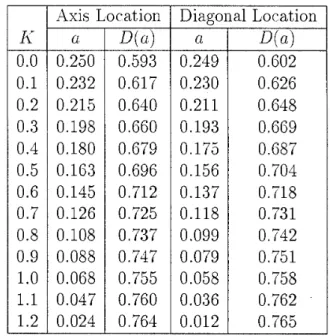
by some algebraic manipulations:

Table 1: Optimal solutions for two hubs in a square Axis Location Diagonal Location

7

where $ ( a ) is defined by ( 2 . 8 ) . For a = 0 I< = 2^/245(1) - 2 = 1.2465, and for K = 1

a = 0.0582.

The two cases were solved for various values of

K .

In all cases the solution on the axis is slightly better than the solution when the hubs are located on the diagonal. The results are presented in Table 1.

Example 3: Three hubs in a square

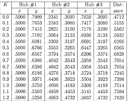
We also experimented with the case of three hubs locat'ed in a square. This example requires the use of the complete formula (2.12) because the Voronoi diagrams change when the locations of the hubs change. The locations of the hubs for various values of

K

are summarized in Table 2 and depicted in Figure 1.

Note that for

K

>_ 1.3 the solution is to locate all three hubs a t the center of the square yielding a distance of 0.7652.

Example 4: Two

hubs

in a rectangle

Assume a rectangle with length b and height 1 / b for b

>

1. Let the two hubs be located

at ( - a , 0 ) a,nd ( a , 0). Then the equivalent equation (2.14) is:

The optimal value of a is determined by the equation:

(2.19)

(2-I<)b

Since +(X) E X for a small :r, this equation reduces to a = _{for a large b. We}

A. Suzuki & 2. Drezner

Table 2: Location of three hubs in a square

Hub #l Hub #2 Hub #3 Dist-

ance

Figure 1: Location of three hubs in a square for different values of K

maxinml

K

is obtained for a = 0:

The limit of as b goes t,o infinity is "2".

3. The Second Model

3.1. Problem formulation

Assume that each customer will use only one hub to get to its destination. That means, that one of the n hubs is selected by the customer, and tlie customer travels to that hub and then travels from that hub to his destination. The objective in selecting a hub is to minimize travel, i.e. the sum of distances from the customer's location to the hub and from the hub to its destination is minimized. Consider first m customers located at

Ai

= (oj,bj)

for 1; = 1,

.

. . ? R . In this case, the objective function to be minimized is:

^LYi

.

+ +

,

-Yn) =

E E

min {d(Xi, As)

+

d(Xi, A,)}

s=1 t = l \<i<n

Note t,hat by this formulation a customer cannot travel directly to its destination but must use a hub airport. When a cont,inuous area is involved, the sums are replaced by integrals and the analysis is similar to that of the first model. In the following we consider the two-hub case. Two cases in a square are analyzed: hubs located on an axis, and hubs located on a diagonal. The square is centered at (0,O). The last case is that hubs are located in a re~ta~ngle.

3.2. The case of hubs located on the axis

When the hubs are on an axis, the sides of the square are parallel t o the axes and the two hubs are located a t (-a, 0) and ( a , 0). Consider a customer located a t ( U , v ) for ? L , v

>

0.

The other three quadrants offer similar results. For some destinations the customer will use the "closer" hub a t (a, 0) and for some others the customer will use the "farther" hub (-a, 0). The boundary between the destinations that use the closer hub and the destinations that use the fart,lier hub is determined by the following equation. Assume a destination ( X , y).

The boundary is the solution to:

Let 2A =

i / ( u

-

4

2

.

Note that by the triangle inequality

A

<

a. This lea8cls to:

;r2

y2

A2 _{a2 - A2} = 1 (3.3)

The calculation of the average travel distance for a given a , U , and

v

(and consequently

a given A ) is now presented. In the area bounded by tlie hyperbola (3.3) (that includes the point ( - 0 ~ 0 ) ) distances to (-a, 0) should be used (because the route via hub (-a, 0) is shorter than tlie route via hub ( a , 0)). and outside this hyperbolic area distances to (a, 0) should be used. It is easier t o integrate using the distances to ( a , 0) over the complete square, and using the difference between the distances t o ( a , 0) and (-a, 0) when integrating over

the hyperbolic region. This leads t o the following formula for tthe average distance D ( a , 21, v )

for a given a . positive quadrant ( U . P ) and consequently a given A:

which leacls to:

The average dista,nce, D ( a ) , is obta,ined by integrating over all posit,ive (U. U):

For a = 0 the formula is simplified because the last integral in (3.4) vanishes and:

v1 7T - - - 4 cos 9 ln(v/2

+

l )

+

v/2

3 = 0.7652. (3.6) 0 0 0

The average distance as a function of c1 is depicted in Figure 2. We used Gaussian quaclrature forn~ulas based on Legendre polynomials with 20 points for the outer three dimensions, and used 48 integration points for the inner dimension (y) [l]. The total number of integration points is therefore 203 . 4 8 = 384,000. Obtaining one value of D(a) took about 10 seconds on a 486 IBM compatible computer.

3.3. The case of hubs located on the diagonal

As before, the square, with area of 1, is cent,erecl at (0.0). The square is rotated by

45'

so it is easier t o construct the equations. The square is defined by the four equations:

&X & y

<:

9.

Let the two hubs be symmetrically located on the x-axis a t ( - 0 , O ) and ( a , 0).

0.00 0.05 0.10 0.15 0.20 0.25 a

Figure 2: The average distance D ( a ) as a function of a in the axis case

The average distance, D ( a ) , is obtained by integrating over all positive ( U , v):

We found the optimal solution for in this case numerically. The optimal location was at a distance of 0.1949 from the center with a minimal average distance of 0.6820. This average distance is better than the average distance of 0.6846 that was obtained for t,he axis location of hubs. This confirms the result in [l51 where it is reported that a solution t o 100 and 200 airports randomly selected in a square was on t,he diagonal of the square a t a distance very close t o the opt,imal location obtained here.

3.4. The rectangle case

Assume that the area is a rectangle of length b and height

i.

The equations can be easily modified t o finding the best location for the hub. In Table 3 we report the best location for

the hub (the minimal point in Figure 2, but for various values of 6 ) . Since the best location and the minimal distance are quite proportional to b, we report in Table 3 those values divided by b. The minimal average distance is about 40% of the rectangle's length for long and narrow rectangles. The best locations for the hubs are about 20% of the rectangle's length from t,lie center.

We approximated the United States by a rectangle and found the locations for two hubs (20% of the length of the rectangle off its center). See Figure

3.

The rectangle was superimposed on the map by free-hand drawing and no calculations were used for its determination. The locations are very close to Indianapolis, Indiana, and quite close t o Denver, Colorado ( a little t o the west of it). United Airline has four major hub airpoits in the United States. These are San Francisco. Denver, Chicago and Washington D. C. Considering San Francisco for transpacific routes and Washington D.

C.

for transatlantic route, their hub airports are quite near t o our results obtained above. (Chicago is approximately 300

A. Suzuki & Z. Drezner

Table 3: Best locat,ion and minimal distance for a recta,ngle

Figure 3: Two Hubs Approxinia,tely Located in the United States

4. Conclusions

The hub selection problem when demand is evenly spread in a given area is formulated and solved. Two formulations are considered. One model assumes that a customer will use two hubs, the one closest to him and the one closest to his destination. A customer will travel t o the closest hub, then to the other hub and then to his destination. The second model assumes that a customer selects only one hub, travels to that hub and then to his destination. The customer selects the hub that provides the shortest total distance t o his destination.

The problem of two hubs to be selected in a square are analyzed. For the first model, the best location for the two hubs is on the axis parallel to the square's side. For the second model the best location is on the diagonal of the square. Both models were also analyzed for a rectangle, and the best axis location is found as a function of the shape of that rectangle. For the first model, three-hub case is also analyzed. The best hub location varied according t o the factor of economy of scale.

References

Abramowitz M. and I.A. Stegun (1972) Handbook of Mathematical Functions, National Bureau of Standards, 9th printing.

Aykin T . (1988) "On the Location of Hub Facilities," Transportation Science, 22, 155- 157.

Drezner Z. and E. Erkut (1995) " Solving the Continuous pDispersion Problem Using

Non-Linear Programming," Journal of the Operational Research Society, 46, 516-520. Drezner

Z.

and E. Zemel (1992) "Competitive Location in the Plane," Annals of Op- erations Research, 40, 173- 193.

Iri M., K. Murota, and T . Ohya (1984) "A fast Voronoi Diagram Algorithm with Appli- cations to Geographical Optimization Problems," Proceedings of the IFIP Conference on System Modelling and Optimization, 1983, Copenhagen, Denmark. Also in System Modelling and Optimization, Lecture Notes in Control and Information Science, Vol. 59, 273-288, P. Thoft-Christensen Ed., Springer-Verlag, Berlin.

Klincewicz J.G. (1991) "Heuristics for the p-Hub Location Problem," European Journal of Operational Research, 53, 25-37.

Klincewicz J.G. (1992) "Avoiding Local Optima in the p-Hub Location Problem Using Tabu Search and GRASP," Annals of Operations Research, 40, 283-302.

Okabe A., B. Boots, and K. Sugihara (1992) Spatial Tesselations - Concepts and Ap- plications of Voronoi Diagrams, John Wiley & Sons, Chichester, England.

Okabe A., and A. Suzuki (1987) "Stability in Spatial Competition for a Large Number of Firms on a Bounded Two-Dimensional Space," Environment and Planning A, 19, 1067-1082.

O'Kelly M.E. (1986) "The Location of Interacting Hub Facilities," Transportation Sci- ence, 20, 92-106.

0 'Kelly M.E. (1986) "Activity Levels at Hub facilities in Interacting Networks," Geo- graphical Analysis, 18, 343-356.

O'Kelly M.E. (1987) "A Quadratic Integer Program for the Location of Interacting Hub facilities," European Journal of Operational Research, 32, 393-404.

74 A. Suzuki & 2. Drezner

[l41 O'Kelly M.E. (1992) "Hub Facility Location with Fixed Costs," Papers in Regional Science, 71, 293-306.

[l51 Sasaki M., A. Suzuki, and Z. Drezner "On the Selection of Hub Airports on the Airline Hub-and Spoke System, " Submitted for publicat ion.

[l61 Sugihara

K., and M. Iri (1992) "Construction of the Voronoi Diagram for "One Million"

Generators in Single-Precision Arithmetic," Proceedings of the IEEE, 80, 1471-1484. [l 71 Sugiha,ra

K.

and M. Iri (1994)

"A

Robust Topology-Oriented Incremental Algorit hrn

for Voronoi Diagrams," International Journal of Computational Geometry and Appli- cations, 4, 179-228.

[l81 Suzuki A. and Z. Drezner (1995) "On the p-Center Problem in an Area," to appear in Location Science.

[l91 Suzuki A. and A. Okabe (1995) "Using Voronoi Diagrams," in Facility Location:

A

survey of Applications and Methods, Z. Drezner (ed.), Springer-Verlag, New York.

Atsuo Suzuki

Department of Information Systems

&

Quantitative Sciences Nanzan University

Nagoya, Aichi, 466 Japan email: [email protected] Zvi Drezner

Department of Management Science/Informat ion Systems California State University-Fullerton

Fullerton, CA 92634