早稲田大学基幹理工研究科
Master’s Thesis 修 士 論 文
Title 論 文 題 目
UE RF Condition Estimation using Machine Learning
2016年7月19
Student ID
学籍番号 5114FG05-1
Name
氏名 Chen Tao
Supervisor
指導教員
嶋本 薫
印Graduation Thesis
UE RF Condition Estimation using Machine Learning
Department of Computer Science and Communications Engineering, School of Fundamental Science and Engineering Waseda University
Tokyo, Japan
SHIMAMOTO shigeru Lab Chen Tao
19, July, 2016
Contents
Acknowledgements
... 4Abstract
... 5§1 Introduction
... 6§1.1 Motivation ... 6
§1.2 Related work ... 6
§1.3 Contribution of the research... 7
§1.4 Organization of the thesis ... 7
§2. Background
... 8§2.1 LTE network system architecture ... 8
§2.1.1 LTE network radio performance ... 10
§2.1.2 Radio frequency parameters ... 11
§2.2 Mobility problem ... 13
§2.2.1 Classification of mobility problem ... 14
§2.2.2 Error evaluation of mobility problem ... 16
§3. Machine learning scheme
... 17§3.1 System architecture ... 17
§3.2 Introduction of machine learning ... 18
§3.3 Learning algorithm... 19
§3.3.1 Linear regression method ... 20
§3.3.2 Logistic regression method ... 23
§3.4 The fitting problems ... 29
§3.4.1 Regularized linear regression ... 30
§3.4.2 Regularized logistic regression ... 31
§4. Numerical Results
... 32§4.1 Performance of Linear Regression Method ... 32
§4.1.1 Linear result in basic features(4 features)... 32
§4.1.2 Linear result in derived features(6 features) ... 34
§4.1.3 Linear result in more additional features(11 features)... 38
§4.2 Performance of Logistic Regression Method ... 42
§4.2.1 Logistic result in basic features(4 features) ... 42
§4.2.2 Logistic result in derived features(6 features) ... 44
§4.2.3 Logistic result in more additional features(11,21 features) ... 46
§4.3 Results Summary ... 53
§4.3.1 Best case of logistic & linear ... 53
§4.3.2 Handover problems analysis ... 58
§5. Conclusion
... 60Appendix I
... 61Appendix II
... 63References
... 66Publication
... 67Acknowledgements
I am grateful to acknowledge many individuals who have helped me to accomplish this research. Firstly, I would like to extend my sincere thanks to my supervisor, Prof.
Shigeru Shimamoto, for the weekly discussions and kind advice and encouragement through my study at FSE Waseda University. His wise advices and kindness have been invaluable and helped the result in great improvement in my research.
I am also very grateful to all my friends in the Shimamoto laboratory, especially Zhenni Pan & Mohamad Erick Ernawan, without all you help I cannot finish all this work.
And finally, my deepest thanks to my parents & sisters, I truly appreciate them and I could not have done this without them. I also thank them for their continuous love and guidance throughout my entire life.
Abstract
Estimating the user equipment (UE) radio frequency (RF) condition will be a key factor to analyze overall network performance. Actual RF estimation based on scanner data log can only observe UE at top-serving cell with good RF condition only. However, a RF potential problem may still occurred since the actual UE possibly located in poor RF condition and not always be served by the top-1 cell regarding the real UE data log which cannot be observed from scanner data log. In this paper, we estimate the UE RF condition assisted by machine learning (ML) using UE data log (in the future we use Scanner data log) and detect the mobility problems. A hypothesis was obtained from learning process through various input of RF condition as an input feature. The numerical results shown that the simple ML method can accurately estimate the UE RF condition.
Keyword
Supervised Machine Learning, RF Condition, Mobility Problem, Estimation.
§1 Introduction
§1.1 Motivation
Future wireless network performance like in 5G will involves “big data” as the data traffic is keep increasing and the network become ubiquitous. Utilizing manual method is impossible to analyze those network conditions with continuous data stream.
Machine learning (ML) can be utilized as a tool to process a very large data set input (ex: UE RF condition) and analyze the network performance. We can estimate the RF condition using different data set. One called UE data log while the other is Scanner data log. Using Scanner data log, we can only observed UE at TOP serving cell with good RF condition[1].
However, based on UE Data Log, actual UE serving cell may not be in good RF condition, thus creating UE RF potential problems. Therefore it is very important to estimate the actual UE RF condition.
Due to the format similarity between UE data and scanner data, we can apply ML to estimate UE RF condition based on the scanner data log (ex: possibility whether UE served by TOP 1 cell or not) and develop the “learn” function or hypothesis[2] to “learn”
the RF condition based on the Nth input (fundamental parameter& derived parameters) from Scanner data log, also the probability of potential mobility problem.
The aim of this article is to introduce the basic idea of the RF estimation algorism with UE log data by ML method. First is detecting the potential performance problems from RF UE data using ML algorithm. Second is providing the probability of problem occurrences using ML.
§1.2 Related work
To complete our article we have to check the previous research firstly. With ML is turning noted,“Self-Aware Network”[3] becomes a hot topic, it could autonomously handle the complex network optimization in real-time. Machine learning algorithms provide signals, patterns and models to predict the network status and to make the right decisions to improve the help from the unstructured big data and event society.
Some other papers mentioned the optimization of session drops[4],the prediction of vehicular traffic and communication connectivity[5].
Also, there is a system which mentioned the machine learning and data mining for
Path-Loss / Radio and Interference Map Reconstruction[6], uplink interference management using ML[7], and wireless Interference segmentation and prediction[8]. Even some paper showed some pure algorithm about "Estimating Probabilities"[9]. Comparing with other studies , we found there is some points that estimate the UE RF condition and probability of mobility problems.
§1.3 Contribution of the research
In this paper, we give an analysis through supervised machine learning with the target of estimating the conflict zone between the scanner data and UE log where a mobility problem may occur. A hypothesis is derived from learning through various kinds of RF features. Finally can be accurately estimated the UE RF condition.
§1.4 Organization of the thesis
In the first chapter I will explain the purpose and objective of the study. Then In the second chapter, I will start from the introduction of LTE networks and network parameters, even the mobility of LTE networks. In the third chapter, I will combine the actual parameters of the study explained ML algorithm, also the solutions for ML training problems. In the fourth chapter, I will show many different results by using Matlab simulator. Lastly I may do the conclusion of the whole study.
§2. Background
§2.1 LTE network system architecture
Fig .1 LTE network architecture[10]
LTE network interfaces:
1) eNodeB - eNodeB: X2 interface 2) eNodeB - MME: S1-MME interface 3) eNodeB - S-GW: S1-U interface 4) MME - MME: S10 interface 5) MME - S-GW: S11 interface LTE network frequency bands:
1) A band: 2010M~2025M 2) D band: 2570M~2620M 3) F band: 1880M~1920M 4) E band: 2300M~2400M
Fig .2 LTE network scenario[11]
The main components of the LTE network, there is E-UTRAN radio network (Evolved Universal Terrestrial Radio Access Network) and the core network EPC (Evolved Packet Core).E-UTRAN is composed of a base station apparatus (eNode B).
The EPC includes, MME (Mobility Management Entity) that function as network control of access gateway control plane; S-GW (Serving Gateway) that function as User-plane of gateway; P-GW (Packet data network Gateway) that function as gateway for connecting to an external of the Internet and corporate intranet.
One of LTE features, unlike the 3G, it has no nodes RNC (Radio Network Controller) which performs a base station controller in a wireless network. It has the advantage that can be performed in simple network , shortening connection delay and transmission delay.
§2.1.1 LTE network radio performance
The key technical requirements and performance:
Fig .3 The key technical requirements and performance Details of LTE network radio performance[12]:
1)Peak data rate:
·Under the conditions of allocation of downlink frequency spectrum,downlink data rate up to 100Mbps.
·Under the conditions of allocation of uplink frequency spectrum, uplink data rate up to 50Mbps.
2)Spectral efficiency:
·Downlink: at full capacity networks, LTE spectral efficiency (with each station site, each Hz, measured by the number of bits per second) goal is 3-4 times of the Release 6 HSDPA.
·Uplink: at full capacity networks, LTE spectral efficiency (with each station site, each Hz, measured by the number of bits per second) goal is 2-3 times of Release 6 enhancements.
3)Mobility:
·E-UTRAN system can optimize the characteristics of mobile users moving at low speed(≤15Km/h).
Enhence cell coverage
DL:100Mbps UL:50Mbps
Reduce delays Lower
OPEX &
CAPEX Support
different bandwidth
s Enhence frequency efficiency
LTE
·Provide a high-performance service for mobile users at the speed of 15-120km/h.
·It can support the mobile user services between the cellular network at the speed of 120-350km/h.
·The situation is higher than 350km/h, the system makes sure user online.
4)Coverage (cell edge bit rate):
·Throughput, spectrum efficiency and mobility indicators within the cell covered by a 5 km radius will be fully guaranteed. When the cell radius increased to 30 km, only bring a slight weakening of the above indicators. At the same time the need to support cell coverage at 100 km above the mobile user services.
5)Other performance indicators:
·Radio resource management requirements:
Enhanced support end to end Quality of Service, Effective support for high-level transmission,
Support the policy management between load sharing and different wireless access technologies.
·Reduce CAPEX and OPEX:
Flatting of architecture and reducing of intermediate nodes make equipment costs and maintenance costs reduce.
§2.1.2 Radio frequency parameters
In our ML method the training data sets are belonging the wireless parameters, therefore the input and the output directly or indirectly have some relation of these radio frequency parameters[13][14]:
1) PCI(physical-layer Cell identity):
·PCI is composed of a primary synchronization signal (PSS) and a secondary synchronization signal (SSS), can be obtained by a simple operation. The following formula: PCI = PSS + 3 * SSS, which PSS a value of 0 ... 2(actually three different sequences PSS), SSS value of 0 ... 167 (actually 168 different sequences SSS),using the above formula available PCI ranges from 0 ... 503, so there is 504 PCI at the physical layer.
·From the view of network operation and maintenance level, CI (Cell Identity) that uniquely identifies a cell in the network which cannot be repeated.
2) RSRP(Reference Signal Receiving Power):
·Reference Signal Receiving Power , transmission power of base station. RSRP units:
dBm.
·RSRP signal strength distribution from the interval:
Table .1 RSRP signal strength distribution RSRP(dBm) Covering
strength level
Remark
Rx<= -105 6 Very poor coverage. Basic service does not work correctly
-105<Rx<=-95 5 Poor coverage. Outdoor voice services could call, but low call success rate, high call drop rate. Indoor basic service operations cannot be
initiated.
-95<Rx<=-85 4 Covering general, outdoor capable of initiating various services available to low-rate data services. But low call success
rate, high call drop rate.
-85<Rx<=-75 3 Better coverage, outdoor can initiate a variety of services, available medium rate data services.Indoor can initiate various services
available to low-rate data services.
-75<Rx<=-65 2 Good coverage, outdoor can initiate various services available to high speed data services.
Indoor can initiate a variety of services, available medium rate data services.
Rx>-65 1 Coverage is very good.
3) RSRQ(Reference Signal Receiving Quality):
·RSRQ, It represents LTE reference signal receiving quality, this measure is mainly to sort different LTE signal quality of candidate cells. This measurement is used as handover and cell reselection decision index data. Calculation method:RSRP = N * RSRP / (LTE carrier wave RSSI), where N is number of LTE carrier wave resource block (RB). RSRQ achieves an efficient way to report the combination of signal strength and interference effects.
·RSSI (Received Signal Strength Indication), indicating the superposition of all UE received signal.
·SRS( Sounding reference signal):
Periodic SRS (corresponding to the trigger type 0), configured by RRC。
Aperiodic SRS (corresponding trigger type 1)eNodeB may send aperiodic SRS by UE.
4) UE transmit power:
·UE maximum transmit power 23dbm, using uplink power control, the transmit power in a good wireless environment condition is small, in a poor wireless
environment condition, t is quite great.
·The PUCCH (physical uplink shared channel), PUCCH (physical uplink control channel), RACH (random access channel).
5) SINR(Signal to Interference plus Noise Ratio):
·SINR in the range between -20 to 30.
·During the test, the test point value requirements:
Table .2 SINR test point value requirements
Point level Rang of RSRP Rang of SINR
Excellent point >-85dBm >25
Good point -85~-95dBm 16-25
Normal point -95~-105dBm 11-15
Poor point -105~-115dBm 3-10
Very poor point <-115dBm <3
6) Transmission mode:TM value, indicating transmission mode
·TM1 represents a single antenna transmitting data.
·TM2 represents transmit diversity(two antennas transmit the same data, in poor case wireless environment (RSRP and SINR difference), is suitable for edge area.
·TM3 indicates the open-loop spatial multiplexing(two antennas transmit different data , rate can be increased by 1 times).
·TM4 represents closed-loop spatial multiplexing.
·TM5 represents multiuser MIMO(Multiple-Input Multiple-Output).
·TM6 represents closed loop pre-coding of rank =1.
·TM7 represents using single antenna port and single-stream BF.
·TM8 represents double-stream BF.
§2.2 Mobility problem
Potential Problems can be categorized into 4 different root causes.
Fig .4 4 different root causes
§2.2.1 Classification of mobility problem
ML need to detect the mobility problems whether its Late/Early handover[15] or wrong handover scenario that leads to potential problems (ex: RLF, Silence VoLTE).
Estimating mobility problem while considering different mobility parameters (eg.
event eA2/eA3/eA4/eA5 including Hys+offset parameters and TTT) can captured those scenarios in the ML process.
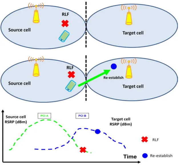
1)Mobility Problems Late Handover:Late handover occurred when RLF happened in source cell before handover initiated
·After RLF UE will try to establish a radio link in target cell.
·Other possibility is RLF in source cell happened during handover procedure and UE attempts reestablish radio link in target cell.
Fig .5 Late handover scenario
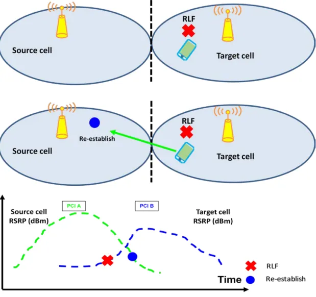
2) Mobility Problems Early Handover: too early handover occurred when RLF happened at target cell after handover process.
·After RLF UE will reestablish its radio link in the source cell.
·Other possibility is RLF happened in the target cell during handover and UE try to reestablish radio link in source cell.
Fig .6 Early handover scenario
3) Mobility Problems Wrong Handover: wrong handover occurred when RLF happened at target cell after handover process.
·After RLF UE will reestablish its radio link not in the source cell or target cell.
·Other possibility is RLF happened in the target cell during handover and UE try to reestablish radio link not in the source cell or target cell.
Fig .7 Wrong handover scenario
§2.2.2 Error evaluation of mobility problem
LTE handover failure analysis: LTE handover type is hard switch.
1)Hardware failure (Base station, UE).
2)Traffic congestion (current LTE network not for the moment).
3)Neighborhood Cell configuration issues.
§3. Machine learning scheme
§3.1 System architecture
In our supervised learning system, firstly we build a training dataset which includes the input and output. According to the original UE data log, inputs include Serving-PCI, TOP1-PCI, Serving-RSRP, Serving-RSRQ, Serving-SINR, TOP1~TOP2 NCell-RSRP, and also the derived features .
To consider about the probability of UE mobility problem, we defined as following:
when Serving-PCI is equal TOP1-PCI, then output becomes"0", means UE has no mobility problem; else output becomes"1", means UE has mobility problem.
Therefore output is set {0,1}. Then after the ML process, we can learn a function H(x) as a “good predictor” of the output. In the future when input the scanner data only with no UE data and get the changing of RF condition, also the potential problem(low throughput, VoLTE mute, radio link failure) would be estimated. Blowing figure is the workflow of the system.
Fig .8 Supervised machine learning procedures
§3.2 Introduction of machine learning
1)Historical development of machine learning[16]
Machine learning is a study about how computer simulation or implementation of interdisciplinary studying human behavior in many fields, involving probability theory, statistics, convex optimization, complexity theory and many other sciences.
The development of machine learning can be divided into four periods:
·Through Learning System
·Concept learning system based notation
·Learning System Based on Knowledge
·Depth study of coupling learning and learning sign 2)Machine learning classification[17]:
·Rote learning
Learner information provided directly to the receiving environment, without reasoning or information transfer.
·Learning from instruction
Students get information from the environment, to turn knowledge into an internal representation that can be used, and the organic combination of new knowledge and existing knowledge as one.
·Learning by deduction
Students form of used reasoning in deductive. Reasoning from kilometers, goes through logical transformation deduce conclusions
·Learning by analogy
Using two different fields of knowledge similarity, by analogy, deriving in response to the target domain knowledge from the source domain knowledge in order to achieve learning
·Explanation-based learning
According target concept provided an example of this concept, the field of theoretical and operational criteria, first construct an explanation as to why this example to meet the target concept, and then explain the position to promote the target concept sufficient condition to meet the operational guidelines
·Learning from induction
Such reasoning workload much more than learning Learning from instruction and Learning by deduction, because the environment does not provide a general description of the concept
§3.3 Learning algorithm
Step1: Initial preparation:
Checking the training data sample to decide the input(x) and output(y) of training sample.
Defined output:If △(Serving PCI - Top1 PCI) = 0, "0" UE has no Mobility problem;
else △(Serving PCI - Top1 PCI) ≠ 0, "1" UE has Mobility problem. Our Y of training samples is set {0,1}
Basic Feature: serving_rsrp, serving_rsrq, serving_sinr, top1NCell_rsrp ~ top6NCell_rsrp
Step2: Training algorithm:
Continuous and discrete output can be categorized as regression and classification problems, respectively.
In ML we propose use linear method and logistic method[18] . Both regression and classification have single and multiple input problems.
Step3: Categorization:
Categorize H(x) value and Y into several groups, calculate average value of each groups, then plot in figures.
Table .3 Example of groups categorization Categorized
Serving-RSRP Range X axis: Serving-RSRP Average of Y
Average of H(x)
(RSRP≤-160) -160 / /
(-160<RSRP≤-150) -150 / /
(-150<RSRP≤-130) -140 / /
(-130<RSRP≤-120) -130 / /
(-120<RSRP≤-115) -120 / /
(-115<RSRP≤-105) -110 / /
(-105<RSRP≤-95) -100 / /
(-95<RSRP≤-85) -90 / /
(-85<RSRP≤-75) -80 / /
(-75<RSRP≤-65) -70 / /
(-65<RSRP) -60 / /
§3.3.1 Linear regression method
1)Linear Regression with multiple features:
Multifeature hypothesis: multi-dimensional input from the output decision that the input of the multi-dimensional features. As shown below: Mobility problems is output to the front of the four-dimensional input.
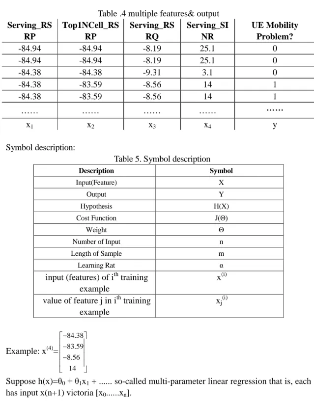
Table .4 multiple features& output Serving_RS
RP
Top1NCell_RS RP
Serving_RS RQ
Serving_SI NR
UE Mobility Problem?
-84.94 -84.94 -8.19 25.1 0
-84.94 -84.94 -8.19 25.1 0
-84.38 -84.38 -9.31 3.1 0
-84.38 -83.59 -8.56 14 1
-84.38 -83.59 -8.56 14 1
…… …… …… …… ……
x1 x2 x3 x4 y
Symbol description:
Table 5. Symbol description
Description Symbol
Input(Feature) X
Output Y
Hypothesis H(X)
Cost Function J(Θ)
Weight Θ
Number of Input n
Length of Sample m
Learning Rat α
input (features) of ith training example
x(i) value of feature j in ith training
example
xj(i)
Example: x(4)=
84.38 83.59 8.56
14
−
−
−
Suppose h(x)=θ0+ θ1x1 + ... so-called multi-parameter linear regression that is, each has input x(n+1) victoria [x0...xn].
0 1 1 2 2
( ) n n
h x x x x (1)
To convenience, define x0=1,(x0(i)
=1);
0 1 2
...
n
x x
x x
x
=
n1
0 1 2
...
n
θ θ θ θ θ
=
n1
(2)
TX
θ =
[
θ θ0 1 θn]
0 1
n
x x
x
(3)
Therefore h x( ) 0 1 1x 2x2 nxn=θTX (4) 2)Gradient descent for multiple features:
The single feature gradient descent learning method:
Previously (n=1):
Repeat{
0
( ) ( )
0 0
1
( )
: 1 ( )
m
i i
i
J
h x y
m
( ) ( )
( )1 1
1
: 1 ( )
m
i i i
i
h x y x
m
(update 0, 1) } New algorithm for the multiple features learning:
New algorithm (n≥1):
loop {
( ) ( )
( )1
: 1 ( )
m
i i i
j j j
i
h x y x
m
( update j for j=0,…,n) }
( ) ( ) ( )
0 0 0
1
( ) ( ) ( )
1 1 1
1
( ) ( ) ( )
2 2 2
1
: 1 ( )
: 1 ( )
: 1 ( )
m
i i i
i m
i i i
i m
i i i
i
h x y x
m
h x y x
m
h x y x
m
……
……
3)Feature Scaling:
It is important to normalize feature, so use the feature scaling, will soon feature all normalized to [-1,1] interval.
Normalization method:xi=(xi-μi)/σi
min
max min
normalization
x x
x x x
= −
− (5)
4) Learning Rate:
In machine learning gradient descent algorithm another key point is that the rate of design: design guidelines is to ensure that each iteration is guaranteed to make the cost function decrease.
Since the learning rate is too large, so that with the increase in the number of iterations, the J(θ) jump greater, causing the situation where J(θ) can not convergent.
Solution: Reduce learning rate
No. of iterations No. of iterations Fig .10 convergent case Fig .11 not convergent case If α is very small, the speed of gradient descent would be slow.
If α is too much great , we may skip the minimum even wont decrease. therefore α needs to be adjusted according to actual situation.
How to choose a α, test
0.001 0.003 0.01 0.03 0.1 0.3 1
5): Stochastic gradient descent(SGD) and Batch gradient descent(BGD)
Selection between stochastic gradient descent(SGD) and batch gradient descent(BGD).
Table .6 Difference between SGD & BGD
Stochastic gradient descent(SGD) Batch gradient descent(BGD) Each iteration of a new sample, will
update θ
After completing the iteration of all samples will update θ The result is close to the local optima The result is Global optimal Iterative speed is fast even the number
of samples is large m> 10⁵
Iterative speed will be extremely slow To sum up the reasons above, the SGD method is better than BGD for our machine learning algorithm
J(θ) J(θ)
§3.3.2 Logistic regression method
Fundamental principles:
··Find a suitable prediction function (hypothesis), generally expressed as H function, which is what we need to find a classification function, it is used to predict the result of the determination of the input data. Critical data needs to have some understanding of when this process or analysis, know or guess "probably" in the form of prediction functions, such as a linear function or nonlinear function
·Constructs a cost function (loss of function), the function indicates a deviation between predictable output (h) and categories of training data (y).
·Obviously, the value of J(θ) function smaller the more accurate the prediction function (i.e. the function h more accurate), so this step needs to be done is to find the minimum value of J(θ) function. Get the minimum functions which have different methods when Logistic Regression achieves some gradient descent.
1) Construct predict function :
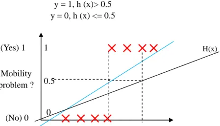
Assumptions linear regression hypothesis of linear equations obtained as shown in the figure above blue line, it can determine a threshold: 0.5 conduct predict
y = 1, if h (x)> = 0.5 y = 0, if h (x) <0.5
Fig .12 Decision case in linear regression 0
H(x)
1
0.5 (Yes) 1
(No) 0 Mobility problem ?
Mobility problem = 0.5 point down the projector, the right of the dot predict y = 1;
left predict y = 0; it can be well classified.Then, if the data set is like this?In this case, it is assumed linear regression which predicts the black line, the boundary of linear equations obtained from 0.5, it can not very well be classified. Because not satisfied
y = 1, h (x)> 0.5 y = 0, h (x) <= 0.5
Fig .13 Linear method cannot make decision case At this point, we introduce the logistic regression model:
Logistic Regression, it is actually a classification method for two classification problems (ie only two output). Need to find a predict function (H), apparently the output of the function must be two values (representing two categories), so we use the logistic function (or called Sigmoid function). The function form is:
( ) 1
1 z
g z e
(6)
Corresponding function image is a value between 0 and 1 S-curve:
Fig .14 S-curve
1
0.5
0 1
0.5 (Yes) 1
(No) 0 Mobility problem ?
H(x)
Non-linear decision boundaries:
Fig .15 Non-linear decision case
2 2
0 1 1 2 2 3 1 4 2
( ) ( )
h x g x x x x (7) Predict ”y=1” if 1 x12x220
In the case of linear boundary, the boundary form follows:
0 1 1
0 n
T
n n i i
i
x x x x
(8) Predict function is:
( ) ( ) 1
1 T
T
h x g x x
e
(9) Value of function hθ(x) has a special meaning, it represents the probability when results were 1, therefore to the input x classification probabilities of the results for Class 1 and Class 0 are as follows:
( 1| ; ) ( )
( 0 | ; ) 1 ( )
P y x h x
P y x h x
(10)
2) Constructs a cost function
Cost function and J(θ) function as a formula of (11) and (12)
log(log(1 ( ))( )) 10Cos ( ( ), )t h x y hhx x if yif y
(11)
( ) ( ) 1
( ) ( ) ( ) ( )
1
( ) 1 Cos ( ( ), )
1 log ( ) (1 ) log(1 ( ))
m
i i
i m
i i i i
i
J t h x y
m
y h x y h x
m
(12)
In fact here Cost functions and J(θ) function is based on derived maximum likelihood.
The following detailed describe the derivation process. With formula(10) together can be written as:
Decision boundaries
( | ; ) ( ( )) (1y ( ))1 y
P y x h x h x (13) Take likelihood function is:
( ) ( )
( ) ( ) 1
( ) ( ) 1
1
( ) ( | ; )
( ( )) i (1 ( )) i
m
i i
i m
i y i y
i
L P y x
h x h x
(14)
Log-likelihood function is:
( ) ( ) ( ) ( )
1
( ) log ( )
log ( ) (1 ) log(1 ( ))
m
i i i i
i
l L
y h x y h x
(15) Maximum likelihood estimation is requested θ when l(θ) takes the maximum value.In fact, here we can use the gradient ascent method for obtaining θ which is optimal parameters.
( ) 1 ( )
J l
m
(16) Because the multiplication of a negative coefficient -1/m, therefore when J(θ) takes the minimum, θ are optimal parameters.
3)Seek minimum of F(θ) by gradient descent
To seek the minimum of J (θ),we can use the gradient descent method, according to the gradient descent method can get the update process of θ:
: ( ), ( 0 )
j j
j
J j n
(17) Where α is learning rate, the following is partial derivative:
( ) ( ) ( ) ( )
( ) ( )
1
1 1 1
( ) ( ) (1 ) ( )
( ) 1 ( )
m
i i i i
i i
j i j j
J y h x y h x
m h x h x
(18)
( ) ( ) ( )
( ) ( )
1
( ) ( ) ( ) ( ) ( )
( ) ( )
1
( ) ( ) ( ) ( ) ( )
1
1 1 1
(1 ) ( )
( ) 1 ( )
1 1 1
(1 ) ( ) 1 ( )
( ) 1 ( )
1 1 ( ) (1 ) ( )
m
i i T i
T i T i
i j
m
i i T i T i T i
T i T i
i j
i T i i T i i
j i
y y g x
m g x g x
y y g x g x x
m g x g x
y g x y g x x
m
( ) ( ) 1
( ) ( ) ( )
1
( ) ( ) ( )
1
1 ( )
1 ( )
1 ( )
m
m
i T i i
j i
m
i i i
j i
m
i i i
j i
y g x x
m
y h x x
m
h x y x
m
The solution procedure used in the following formula:
( )
( ) ( ) 2
( )
( ) ( )
( ) 1 1
( ) 1 ( )
(1 )
1 ( )
1 1
( )(1 ( )) ( )
g x
g x g x
g x
g x g x
f x e
f x e g x
x e x
e g x
e e x
f x f x g x
x
(19)
Thus, the update process can be written as:
( ) ( )
( )1
: 1 ( ) , ( 0 )
m
i i i
j j j
i
h x y x j n
m
(20) Because originally where α is a constant, the 1/m will generally be omitted, so the final θ update process:
( ) ( )
( )1
: ( ) , ( 0 )
m
i i i
j j j
i
h x y x j n
(21) With a maximum of gradient ascent l( ) log ( )L can be obtained:
( ) ( )
( )1
: ( )
( ) , ( 0 )
j j
j m
i i i
j j
i
y h x x j n
(22)
Observed above formula, gradient ascent method and gradient descent algorithm is exactly the same.
4) Vectorized gradient descent process
In order to implement the algorithm in matlab, we have to achieve vectorlization by vector or matrix. The simplest method is:
( ) ( )
( )1
: 1 ( ) , ( 0 )
m
i i i
i
h x y x j n
m
(23) Agreed training data matrix form as follows, x is each row of a training sample,and each column is a different feature values.
(1) (1) (1)
(1) (1)
0 1
(2) (2) (2)
(2) (2)
0 1
( ) ( ) ( )
( ) ( )
0 1
,
n n
m m m
m m
n
x x x
x y
x x x
x y
x y
x x x
x y
(24)
Agreed to form a matrix of the unknown parameter θ is:
0 1
n
(25)
Firstly seek x & θ denoted as A:
(1) (1) (1) (1) (1) (1)
0 1 0 0 0 1 1
(2) (2) (2) (2) (2) (2)
0 1 1 0 0 1 1
( ) ( ) ( ) ( ) ( ) ( )
0 1 0 0 1 1
n n n
n n n
m m m m m m
n n n n
x x x x x x
x x x x x x
A x
x x x x x x
(26)
Seeking hθ(x)-y and denoted as E:
(1) (1) (1)
(2) (2) (2)
( ) ( ) ( )
( )
( )
( ) ( )
( m ) m m
g A y e
g A y e
E h x y g A y
g A y e
(27)
Parameter A in g(A) is a vector, so the function to support the realization of g column vector as an argument and returns a column vector. From the above equation hθ(x)-y once can be calculable by the g(A)-y.
Therefore the θ update process will be:
( ) ( ) ( )
: ( )
0 0 0
1
( ) ( )
0 0
1
(1) (2) ( )
( , , )
0 0 0 0
m i i i
h x y x
i
m i i
e x i
x x x m E
(28)
As the same we can write θj :
(1) (2) ( )
: ( , , m )
j j xj xj xj E
(29) Comprehensive up:
(1) (2) ( )
0 0 0 0 0
(1) (2) ( )
1 1 1 1 1
(1) (2) ( )
:
m m
m
n n n n n
T
x x x
x x x
E
x x x
x E
(30)
It can also be written to:
: 1 xT g x y
m
(31)
§3.4 The fitting problems
Overfitting:
1) simple to understand training samples obtained output and the expected output are basically the same, but the desired output test samples and test samples of the output difference is great.
2) In order to obtain a consistent hypothesis leaving hypothesis becomes overly complex called overfitting.
Imagine some learning algorithm to generate a classifier overfitting, this classification can be one hundred percent correct classification of sample data (ie, shouting sample document to give it, it will never divide wrong), but also to be able to the sample is completely correct classification, so that its structure is so elaborate, strict rules so that any sample data slightly different documents that it does not consider all fall into this category.
Underfitting:
If the data itself is presented quadratic, so with a quadratic curve fit better. But only using a linear equation for fitting purposes. This results in inadequate fitting that is
"under fit" phenomenon, so that when the forecast to result in bias. If we use artificial neural network fitting, because the three-fitting artificial neural network capability which can fit any function. If the fit completely, even experimental data points will be unevenly distributed, the experimental data error etc. "noise" are by least squares fitting criterion into the mathematical model. This of course will result in deviation of forecasts.
Fig .16 3 different fitting situations
Underfitting: obviously there are not caught model structure, for example, the leftmost Figure.
Overfitting: rightmost is an example of over-fitting.
Leftmost function is:
h(x)=01x (32)
The middle added an extra feature x2 ,better fit the data. Function is:
2
0 1 2
( )
h x x x (33)
It seems we add more features, the better the fit; features but adding too much is dangerous, the rightmost figure is a fifth-order polynomial, Although a good fit for a given data set, but this is not a good predictor of function. Function is:
2 3 4 5
0 1 2 3 4 5
( )
h x x x x x x (34) Therefore, selective characteristic for the learning algorithm performance is very important.
How to solve the over-fitting problem? Two methods:
1) Reduce the number of feature (a feature manually define how many remain, these algorithms select feature)
2) The normalized (leaving all feature, but for some feature defines its parameter is very small)
§3.4.1 Regularized linear regression
For θ0, no penalty terms, the same as with the original update formula For other θj, J(θ)on its rear plus a derivation (λ/m)*θj, see below:
Gradient descent:
Loop{
( ) ( )
( )0 0 0
1
: 1 ( )
m
i i i
i
h x y x
m
(35)
1 ( ) ( ) ( )
: [ ( ) ]
1 0
( 1, 2, 3, , )
m i i i
h x y x
j j mi m j
j n
(36)
( ) ( )
( )1
: 1 1 ( )
m
i i i
j j j
i
h x y x
m m
(37) }
If do not use the gradient descent method (gradient descent + regularization), but with the matrix calculation (normal equation) to seek θ, will seek to makeθ of, so that J (θ) for all derivatives Derivative θj is equal to 0, have the following formula:
Assume m training samples( )n features( ), (X XT ) 1X yT
(38) if 0,
1
0 1
( 1 )
1
T T
X X X y
(39)
And has proved something in parentheses in the above formula is reversible.
§3.4.2 Regularized logistic regression
Just same as linear regression, we give J(θ) with respect to θ added penalty term to curb over-fitting.
Gradient decent:
Loop{
( ) ( )
( )0 0 0
1
: 1 ( )
m
i i i
i
h x y x
m
(40)
1 ( ) ( ) ( )
: ( )
1
( 1, 2, 3, , )
m i i i
h x y x
j j mi j m j
j n
(41)
}
Here we find, in fact, it is the same with linear regression θ update method.
§4. Numerical Results
In this chapter, we applied the machine learning algorithm and coded in the Matlab simulator. The results will be different because of the different training features(4,6,11…). Also in the same training features case if the plot X axis changes the curve of result should be changed into different shapes.
§4.1 Performance of Linear Regression Method
§4.1.1 Linear result in basic features(4 features)
4 Features:
1)Serving-RSRP 2) Serving-RSRQ 3) Serving-SINR 4) Top1NCell-RSRP
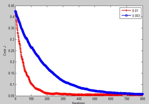
Relation between cost function J(θ) and iterations(4features) is shown as the figure 17. When α=0.01 or 0.003, the J(θ) becomes convergent fast and smoothly. When α turning bigger the speed of convergence is becoming faster. Therefore this will be a reference when we choose the convenient value of α.
Fig .17 Cost function J(θ) convergence(4 features)
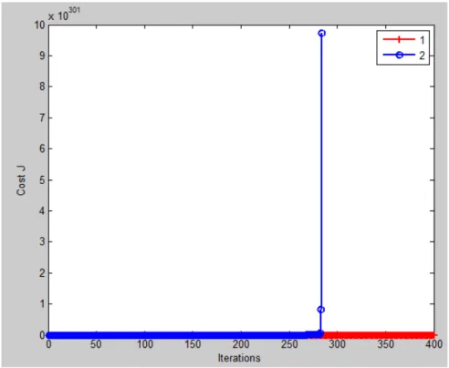
However in figure 18, we found that when α > 1 the cost function J(θ) will be
divergence. Therefore our α should be less than 1 , when we do the training.
Fig .18 Cost function J(θ) is divergence(4 features) Linear Regression Method (4 features):
Plot at X axis: Severing-RSRP
Fig .19 Linear method plotted at Severing-RSRP(4 features)
§4.1.2 Linear result in derived features(6 features)
6 Features:
1) Serving-RSRP 2) Serving-RSRQ 3) Serving-SINR 4) Top1NCell-RSRP
5) Tag1: (丨serving rsrp —top1NCell rsrp丨> 2 threshold)
If (丨serving rsrp—top1NCell rsrp丨) > 2, Tag1 "1"; (2 is the Threshold) else Tag1 "0"
so the Tag1 is metric set {0,1}
6) Tag2: (丨top1NCell rsrp —top2NCell rsrp丨> 2 threshold)
If (丨top1NCell rsrp —top2NCell rsrp丨)> 2, Tag2 "1"; (2 is the Threshold) else Tag2 "0"
so the Tag2 is metric set {0,1}
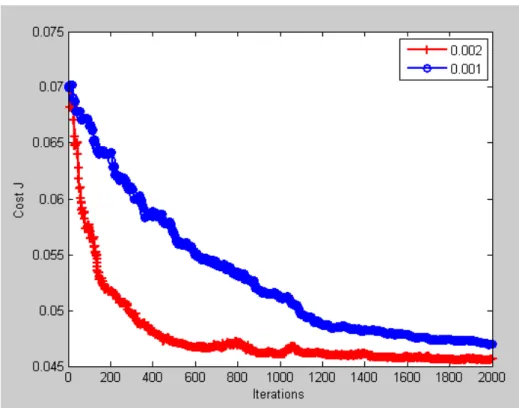
Relation between cost function J(θ) and iterations(6features)
Fig .20 Cost function J(θ) convergence(6 features)
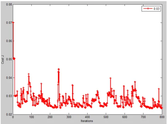
Fig .21 Cost function J(θ) is divergence(6 features)
Linear Regression Method (6 features):
1) Plot at X axis: Severing-RSRP
Fig .22 Linear method plotted at Severing-RSRP(6 features)
Linear Regression Method (6 features):
2) Plot at X axis: Severing-RSRP(categorized in other way)
Fig .23 Linear method plotted at Severing-RSRP(6 features)
Linear Regression Method (6 features):
3) Plot at X axis: Severing-RSRQ
Fig .24 Linear method plotted at Severing-RSRQ(6 features)
Linear Regression Method (6 features):
4)Plot at X axis: Tag1(Serving RSRP - Top1 NCell RSRP)
Fig .25 Linear method plotted at Tag1 (6 features)
Linear Regression Method (6 features):
5)Plot at X axis: Tag2(Top1 NCell RSRP - Top2 NCell RSRP)
Fig .26 Linear method plotted at Tag2 (6 features)
§4.1.3 Linear result in more additional features(11 features)
11 Features:
1) Serving-RSRP 2) Serving-RSRQ 3) Serving-SINR 4) Top1NCell-RSRP
5) Tag1: (丨serving rsrp —top1NCell rsrp丨> 2 threshold) 6) Tag2: (丨top1NCell rsrp —top2NCell rsrp丨> 2 threshold)
7) Tag3: Tag3(New ServingPCI- Old ServingPCI), in every 100ms (every row) mobility problem happened times
If (New ServingPCI- Old ServingPCI) = 0, "0" ; in 100ms mobility problem happened 0 time.
else (New ServingPCI- Old ServingPCI) ≠ 0, "1" ; in 100ms mobility problem happened 1 time.
So the Tag3 is metric set {0,1}
8)Tag4: (New ServingPCI- Old ServingPCI),in every 700ms (every 7 rows) mobility problem happened times
After Normalization So After normalization Tag4∈[0,1].
9) Tag5: Serving_RSRP, in every 700ms (every 7 rows) △(Serving_RSRPEnd - Serving_RSRPHead)
After Normalization
So After normalization Tag5∈[0,1].
min
max min
norm
X X
X X X
= −
−
min
max min
norm
X X
X X X
= −
−
-83.63-(-84.06)=0.43 0.43 0.498120522
10) Tag6: Serving_RSRQ in every 700ms (every 7 rows) △(Serving_RSRQEnd - Serving_RSRQHead)
After Normalization
So After normalization Tag6∈[0,1]
11)Srving_gfactor(Best condition in SINR) ∈(6,30].
Relation between cost function J(θ) and iterations(11features)
Fig .27 Cost function J(θ) convergence(11 features)
min
max min
norm
X X
X X X
= −
−
Fig .28 Cost function J(θ) is divergence(11 features)
Linear Regression Method (11 features):
1) Plot at X axis: Severing-RSRP
Fig .29 Linear method plotted at Severing-RSRP(11 features)
![Fig .3 The key technical requirements and performance Details of LTE network radio performance [12] :](https://thumb-ap.123doks.com/thumbv2/123deta/9853945.1898542/11.892.266.628.311.671/fig-technical-requirements-performance-details-network-radio-performance.webp)